13 Register Allocation

ABSTRACT

The code generated by a compiler must make effective use of the limited resources of the target processor. Among the most constrained resources is the set of hardware registers. Register use plays a major role in determining the performance of compiled code. At the same time, register allocation--the process of deciding which values to keep in registers--is a combinatorially hard problem.

Most compilers decouple decisions about register allocation from other optimization decisions. Thus, most compilers include a separate pass for register allocation. This chapter begins with local register allocation, as a way to introduce the problem and the terminology. The bulk of the chapter focuses on global register allocation and assignment via graph coloring. The advanced topics section discusses some of the many variations on that technique that have been explored in research and employed in practice.

Keywords

Register Allocation, Register Spilling, Copy Coalescing, Graph-Coloring Allocators

13.1 Introduction

Registers are a prominent feature of most processor architectures. Because the processor can access registers faster than it can access memory, register use plays an important role in the runtime performance of compiled code. Register allocation is sufficiently complex that most compilers implement it as a separate pass, either before or after instruction scheduling.

The register allocator determines, at each point in the code, which values will reside in registers and which will reside in memory. Once that decision is made, the allocator must rewrite the code to enforce it, which typically adds load and store operations to move values between memory and specific registers. The allocator might relegate a value to memory because the code contains more live values than the target machine's register set can hold. Alternatively, the allocator might keep a value in memory between uses because it cannot prove that the value can safely reside in a register.

Conceptual Roadmap

A compiler's register allocator takes as input a program that uses some arbitrary number of registers. The allocator transforms the code into an equivalent program that fits into the finite register set of the target machine. It decides, at each point in the code, which values will reside in registers and which will reside in memory. In general, accessing data in registers is faster than accessing it in memory.

Spill When the allocator moves a value from a register to memory, it is said to spill the value.

To transform the code so that it fits into the target machine's register set, the allocator inserts load and store operations that move values, as needed, between registers and memory. These added operations, or "spill code," include loads, stores, and address computations. The allocator tries to minimize the runtime costs of these spills and restores.

Restore When the allocator retrieves a previously spilled value, it is said to restore the value.

As a final complication, register allocation is combinatorially hard. The problems that underlie allocation and assignment are, in their most general forms, NP-complete. Thus, the allocator cannot guarantee optimal solutions in any reasonable amount of time. A good register allocator runs quickly--somewhere between $\mathbf{O}(n)$ and $\mathbf{O}(n^2)$ time, where $n$ is the size of the input program. Thus, a good register allocator computes an effective approximate solution to a hard problem, and does it quickly.

Few Words About Time

The register allocator runs at compile time to rewrite the almost-translated program from the IR program's name space into the actual registers and memory of the target ISA. Register allocation may be followed by a scheduling pass or a final optimization, such as a peephole optimization pass.

The allocator produces code that executes at runtime. Thus, when the allocator reasons about the cost of various decisions, it makes a compile-time estimate of the expected change in running time of the final code. These estimates are, of necessity, approximations.

A few compiler systems have included description-driven, retargetable register allocators. To reconfigure these systems, the compiler writer builds a description of the target machine at design time; build-time tools then construct a working allocator.

Overview

Virtual register a symbolic register name that the compiler uses, before register allocation We write virtual registers as $V{R}_i$ , for $i\ge 0$

To simplify the earlier phases of translation, many compilers use an IR in which the name space is not tied to either the address space of the target processor or its register set. To translate the IR code into assembly code for the target machine, these names must be mapped onto the hardware resourcesof the target machine. Values stored in memory in the IR program must be turned into runtime addresses, using techniques such as those described in Section 7.3. Values kept in virtual registers (VRs) must be mapped into the processor's physical registers (PRs).

Physical register an actual register on the target processor We write physical registers as $P{R}_i$ , for $i\ge 0$.

The underlying memory model of the IR program determines, to a large extent, the register allocator's role (see Section 4.7.1).

• With a register-to-register memory model, the IR uses as many VRs as needed without regard for the size of the PR set. The register allocator must then map the set of VRs onto the set of PRs and insert code to move values between PRs and memory as needed.
• With a memory-to-memory model, the IR keeps all program values in memory, except in the immediate neighborhood of an operation that defines or uses the value. The register allocator can promote a value from memory to a register for a portion of its lifetime to improve performance.

Thus, in a register-to-register model, the input code may not be in a form where it could actually execute on the target computer. The register allocator rewrites that code into a name space and a form where it can execute on the target machine. In the process, the allocator tries to minimize the cost of the new code that it inserts. By contrast, in a memory-to-memory model, all of the data motion between registers and memory is explicit; the code could execute on the target machine. In this situation, allocation becomes an optimization that tries to keep some values in registers longer than the input code did.

Graph coloring an assignment of colors to the nodes of a graph so that two nodes, $n1$ and $n2$ , have different colors if the graph contains the edge $(n1,n2)$.

This chapter focuses on global register allocation in a compiler with a register-to-register memory model. Section 13.3 examines the issues that arise in a single-block allocator; that local allocator, in turn, helps to motivate the need for global allocation. Section 13.4 explores global register allocation via graph coloring. Finally, Section 13.5 explores variations on the global coloring scheme that have been discussed in the literature and tried in practical compilers.

13.2 Background

The design and implementation of a register allocator is a complex task. The decisions made in allocator design may depend on decisions made earlier in the compiler. At the same time, design decisions for the allocator may dictate decisions in earlier passes of the compiler. This section introduces some of the issues that arise in allocator design.

13.2.1 A Name Space for Allocation: Live Ranges

At its heart, the register allocator creates a new name space for the code. It receives code written in terms of Vrs and memory locations; it rewrites the code in a way that maps those Vrs onto both the physical registers and some additional memory locations.

To improve the efficiency of the generated code, the allocator should minimize unneeded data movement, both between registers and memory, and among registers. If the allocator decides to keep some value $x$ in a physical register, it should arrange, if possible, for each definition of $x$ to target the same PR and for each use of $x$ to read that PR. This goal, if achieved, eliminates unneeded register-to-register copy operations; it may also eliminate some stores and loads.

Live range a closed set of related definitions and uses Most allocators use live ranges as values that they consider for placement in a physi- cal register or in memory.

Most register allocators construct a new name space: a name space of live ranges. Each live range (LR) corresponds to a single value, within the scope that the allocator examines. The allocator analyzes the flow of values in the code, constructs its set of LRs, and renames the code to use LR names. The details of what constitutes an LR differ across the scope of allocation and between different allocation algorithms.

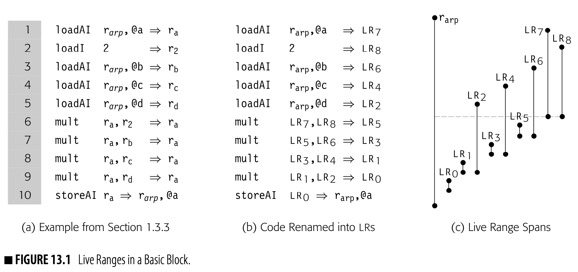
In a single block, LRs are easy to visualize and understand. Each LR corresponds to a single definition and extends from that definition to the value's last use. Fig. 13.1(a) shows an ILOC fragment that appeared in Chapter 1; panel (b) shows the code renamed into its distinct live ranges. The live ranges are shown as a graph in panel (c). The graph can be summarized as a set of intervals; for example LR${}_2$ is [6, 9] and LR${}_8$ is [3, 6]. The drawing in panel (c) assumes no overlap between execution of the operations.

We denote LR${}_8$ as starting in operation three because the operation reads its arguments at the start of its execution and writes its result at the end of its execution. Thus, LR${}_8$ is actually defined at the end of the second operation. By convention, we mark a live range as starting with the first operation after it has been defined. This treatment makes clear that the two instances of $r_1$ in addI $r_1$, $10\Rightarrow r_1$ are not the same live range, unless other context makes them so.

An LR ends for one of two reasons. An operation may be the name's last use along the current path through the code. Alternatively, the code might redefine the name before its next use, to start a new LR.

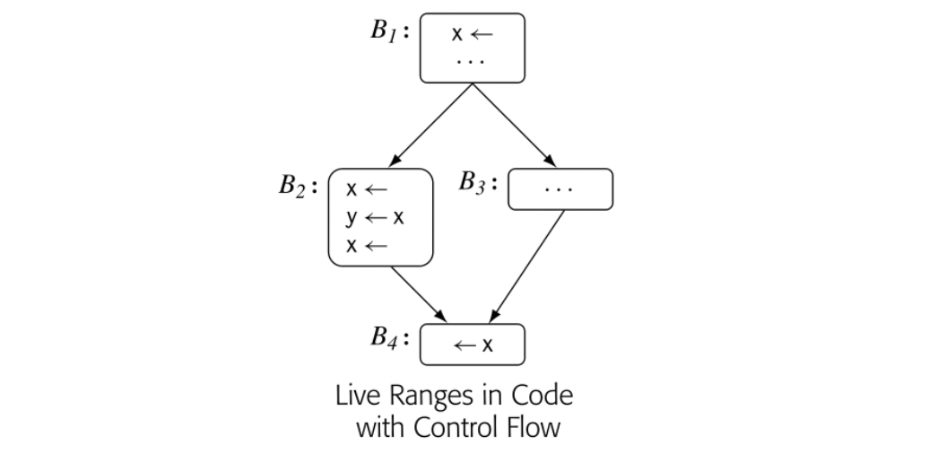
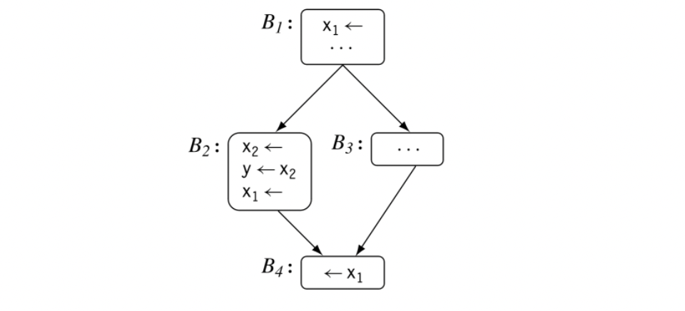
In a CFG with control flow, the situation is more complex, as shown in the margin. Consider the variable x. Its three definitions form two separate and distinct live ranges.

1. The use in $B_4$ refers to two definitions: the one in $B_1$ and the one at the bottom of $B_2$. These three events create the first LR, denoted LR1. LR1 spans $B_1$, $B_3$, $B_4$, and the last statement in $B_2$.
2. The use of x in $B_2$ refers only to the definition that precedes it in $B_2$. This pair creates a second LR, denoted LR2. LR1 and LR2 are independent of each other.

With more complex control flow, live ranges can take on more complicated shapes. In the global allocator from Section 13.4, an LR consists of all the definitions that reach some use, plus all of the uses that those definitions reach. This collection of definitions and uses forms a closed set. The interval notation, which works well in a single block, does not capture the complexity of this situation.

Variations on Live Ranges

The live ranges are as long as possible, given the accuracy of the underlying analysis. More precise information about ambiguity might lengthen some live ranges.

Different allocation algorithms have defined live range in distinct ways. The local allocator described in Section 13.3 treats the entire lifetime of a value in the basic block as a single live range; it uses a maximal-length live range within the block. The global allocator described in Section 13.4 similarly uses a maximal-length live range within the entire procedure.

Other allocators use different notions of a live range. The linear scan allocators use an approximation of live ranges that overestimates their length but produces an interval representation that leads to a faster allocator. The SSA-based allocators treat each SSA name as a separate live range; they must then translate out of SSA form after allocation. Several allocators have restricted the length of live ranges to conform to features in the control-flow

Code Shape and Live Ranges

For the purposes of this discussion, a variable is scalar if it is a single value that can fit into a register.

The register allocator must understand when a source-code variable can legally reside in a register. If the variable is ambiguous, it can only reside in a register between its creation and the next store operation in the code (see Section 4.7.2). If it is unambiguous and scalar, then the allocator can choose to keep it in a register over a longer period of time.

The compiler has two major ways to determine when a value is unambiguous. It can perform static analysis to determine which values are safe to keep in a register; such analysis can range from inexpensive and imprecise through costly and precise. Alternatively, it can encode knowledge of ambiguity into the shape of the code.

If the compiler uses a register-to-register memory model, it can allocate a VR to each unambiguous value. If the VR is live after the return from the procedure that defines it, as with a static value or a call-by-reference parameter, it will also need a memory home. The compiler can save the VR at the necessary points in the code.

If the IR uses a memory-to-memory model, the allocator will still benefit from knowledge about ambiguity. The compiler should record that information with the symbol table entry for each value.

13.2.2 Interference

Interference Two live ranges $L{R}_1$ and $L{R}_2$ interfere if there exists an operation where both are live, and the compiler cannot prove that they have the same value.

The register allocator's most basic function is to determine, for two live ranges, whether or not they can occupy the same register. Two LRs can share a register if they use the same class of register and they are not simultaneously live. If two LRs use the same class of register, but there exists an operation where both LRs are live, then those LRs cannot use the same register, unless the compiler can prove that they have the same value. We say that such live ranges interfere.

Two LRs that use physically distinct classes of registers cannot interfere because they do not compete for the same resource. Thus, for example, a floating-point LR cannot interfere with an integer LR on a processor that uses distinct registers for these two kinds of values.

In the example CFG in the margin, the two LRs for x do not interfere; x2 is only live inside ${\beta }_2$, in a stretch of code where x1 is dead. Thus, the allocation decisions for x1 and x2 are independent. They could share a PR, but there is no inherent reason for the allocator to make that choice.

Interference graph a graph $G=(N,E)$ that has a node n for each LR and an edge $\left(L_R,L_i\right)$ if and only if $L{R}_i$ and $L{R}_j$ interfere

Global allocators operate by finding interferences and using them to guide the allocation process. The allocator described in Section 13.4 builds a concrete representation of these conflicts, an interference graph, and constructs a coloring of the graph to map live ranges onto Prs. Many global allocators follow this paradigm; they vary in the graph's precision and the specific coloring algorithm used.

Finding Interferences

To discover interferences, the compiler first computes live information for the code. Then, it visits each operation in the code and adds interferences. If the operation defines $L{R}_{\mathrm{i}}$, the allocator adds an interference to every $L{R}_j$ that is live at that operation.

The one exception to this rule is a copy operation, $L{R}_{\mathrm{i}}\leftarrow L{R}_{\mathrm{j}}$ which sets the value of $L{R}_{\mathrm{i}}$ to the value of $L{R}_{\mathrm{j}}$. Because the source and destination LRs have the same value, the copy operation does not create an interference between them. If $L{R}_{\mathrm{i}}$ and $L{R}_{\mathrm{j}}$ do not otherwise interfere, they could occupy the same PR.

Interference and Register Pressure

Register pressure a term often used to refer to the demand for registers

The interference graph provides a quick way to estimate the demand for registers, often called register pressure. For a node $L{R}_{\mathrm{i}}$ in the graph, the degree of $L{R}_{\mathrm{i}}$, written $L{R}_{\mathrm{i}}^{\circ }$, is the number of neighbors that $L{R}_{\mathrm{i}}$ has in the graph. If all of $L{R}_{\mathrm{i}}$'s neighbors are live at the same operation, then $L{R}_{\mathrm{i}}^{\circ }+1$ registers would be needed to keep all of these values in registers. If those values are not all live at the same operation, then the register pressure may be lower than the degree. Maximum degree across all the nodes in the interference graph provides a quick upper bound on the number of registers required to execute the program without any spilling.

Representing Physical Registers

Often, the allocator will include nodes in the interference graph to represent Prs. These nodes allow the compiler to specify both connections to PRs and interferences with Prs. For example, if the code passes $L{R}_{\mathrm{i}}$ as the second parameter at a call site, the compiler could record that fact with a copy from $L{R}_{\mathrm{i}}$ to the PR that will hold the second parameter.

Pseudointerference If the compiler adds an edge between $L{R}_i$ and $P{R}_j$, it must recognize that the edge does not actually contribute to demand for registers.

Some compilers use Prs to control assignment of an LR. To force $L{R}_{\mathrm{i}}$ into $P{R}_{\mathrm{j}}$, the compiler can add a pseudointerference from $L{R}_{\mathrm{i}}$ to every PR except $P{R}_{\mathrm{j}}$. Similarly, to prevent $L{R}_{\mathrm{i}}$ from using $P{R}_{\mathrm{j}}$, the compiler can add an interference between $L{R}_{\mathrm{i}}$ and $P{R}_{\mathrm{j}}$. While this mechanism works, it can become cumbersome. The mechanism for handling overlapping register classes presented in Section 13.4.7 provides a more general and elegant way to control placement in a specific PR.

13.2.3 Spill Code

When the allocator decides that it cannot keep some LR in a register, it must spill that LR to memory before reallocating its PR to another value. It must also restore the spilled LR into a PR before any subsequent use. These added spills and restores increase execution time, so the allocator should insert as few of them as practical. The most direct measure of allocation quality is the time spent in spill code at runtime.

Allocators differ in the granularity with which they spill values. The global allocator described in Section 13.4 spills the entire live range. When it decides to spill LR, it inserts a spill after each definition in LR and a restore immediately before each use of LR. In effect, it breaks LR into a set of tiny Lrs, one at each definition and each use.

By contrast, the local allocator described in Section 13.3 spills a live range only between the point where its PR is reallocated and its next use. Because it operates in a single block, with straight-line control flow, it can easily implement this policy; the LR has a unique next use and the point of spill always precedes that use.

Between these two policies, "spill everywhere" and "spill once," lie many possible alternatives. Researchers have experimented with spilling partial live ranges. The problem of selecting an optimal granularity for spilling is, undoubtedly, as hard as finding an optimal allocation; the correct granularity likely differs between live ranges. Section 13.5 describes some of the schemes that compiler writers and researchers have tried.

Nonuniform Spill Costs

To further complicate spilling, the allocator should account for the fact that properties of an LR can change the cost to spill it and to restore it.

An LR might be clean due to a prior spill along the current path, or because its value also exists in memory.

Dirty ValueIn the general case, the LR contains a value that has been computed and has not yet been stored to memory; we say that the LR is dirty. A dirty LR requires a store at its spill points and a load at its restore points.

Clean Value If the LR's value already exists in memory, then a spill does not require a store; we say that the LR is clean. A clean LR costs nothing to spill; its restores cost the same as those of a dirty value.

Rematerializable Value Some Lrs contain values that cost less to recompute than to spill and restore. If the values used to compute the LR'svalue are available at each use of the LR, the allocator can simply recompute the LR's value on demand. A classic example is an LR defined by an immediate load. Such an LR costs nothing to spill; to restore it, the compiler inserts the recomputation. Typically, an immediate load is cheaper than a load from memory.

The allocator should, to the extent possible, account for the nonuniform nature of spill costs. Of course, doing so complicates the allocator. Furthermore, the NP-complete nature of allocation suggests that no simple heuristic will make the best choice in every situation.

Spill Locations

Spill location a memory address associated with an LR that holds its value when the LR has no PR

When the allocator spills a dirty value, it must place the value somewhere in memory. If the LR corresponds precisely to a variable kept in memory, the allocator could spill the value back to that location. Otherwise, it must reserve a location in memory to hold the value during the time when the value is live and not in a PR.

Note that any value in a spill location is unambiguous, an important point for postal- location scheduling.

Most allocators place spill locations at the end of the procedure's local data area. This strategy allows the spill and restore code to access the value at a fixed offset from the ARP, using an address-immediate memory operation if the ISA provides one. The allocator simply increases the size of the local data area, at compile time, so the allocation incurs no direct runtime cost.

Because an LR is only of interest during that portion of the code where it is live, the allocator has the opportunity to reduce the amount of spill memory that it uses. If LR and LR do not interfere, they can share the same spill location. Thus, the allocator can also use the interference graph to color spill locations and reduce memory use for spills.

13.2.4 Register Classes

Register class a distinct group of named registers that share common properties, such as length and supported operations

Many processors support multiple classes of registers. For example, most ISAs have a set of general purpose registers (GPRs) for use in integer operations and address manipulation, and another set of floating-point registers (FPRs). In the case of GPRs and FPRs, the two register classes are, almost always, implemented with physically and logically disjoint register sets.

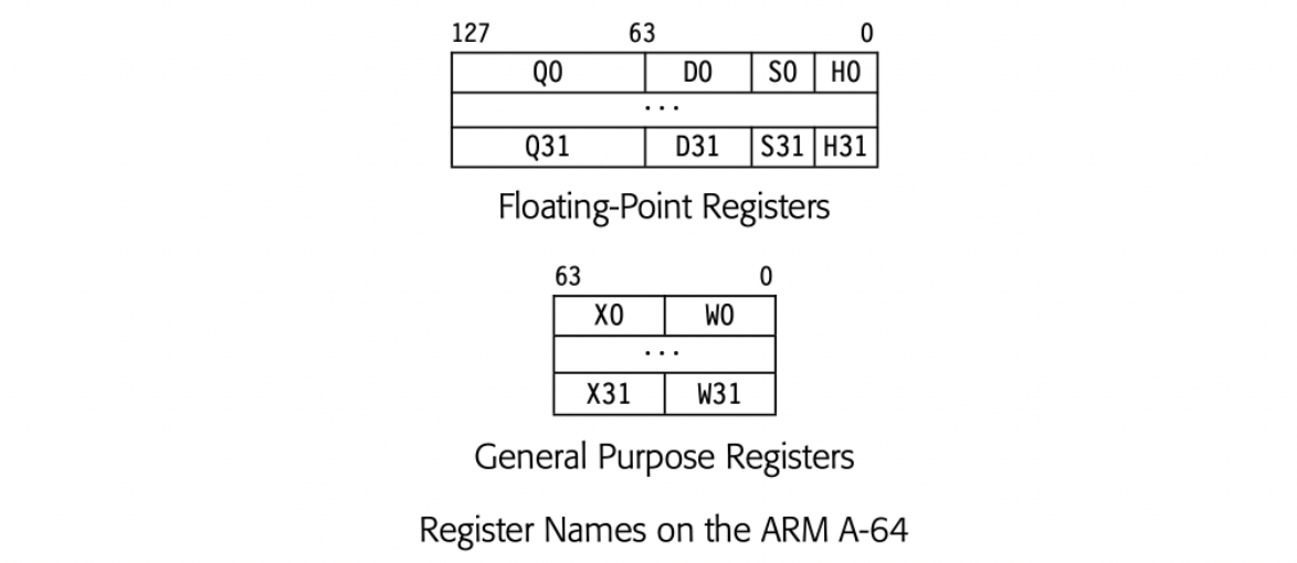
Often, an ISA will overlay multiple register classes onto a single physical register set. As shown in Fig. 13.2(a), the ARM A-64 supports four sizes of floating-point values in one set of quad-precision (128 bit) FPRs. The 128-bit FPRs are named $Q0,Q1,...,Q31$. Each Qi is overlaid with a 64-bit register $Di$, a 32-bit register Si, and a 16-bit register Hi. The shorter registers occupy the low-order bits of the longer registers.

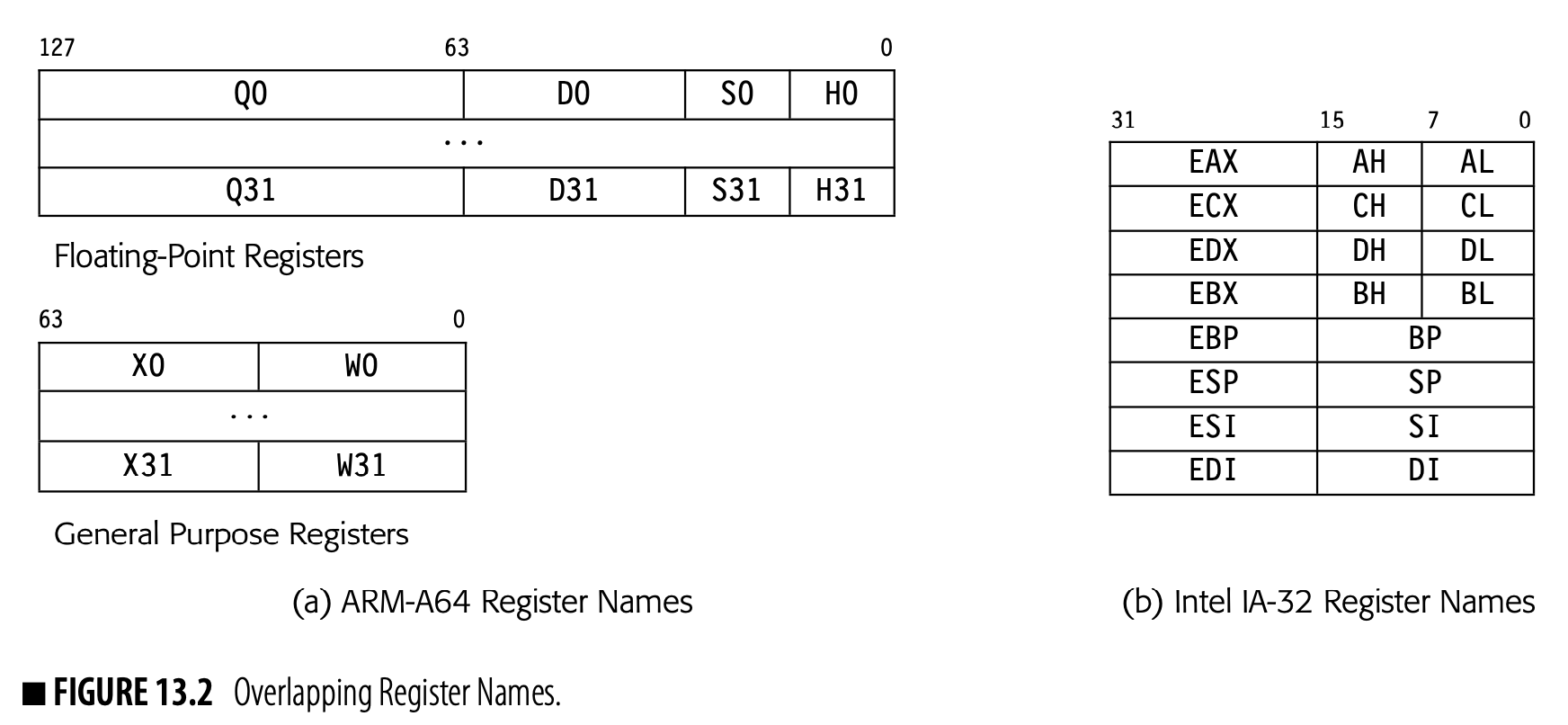
The ARM A-64 GPRs follow a similar scheme. The 64-bit GPRs have both 64-bit names Xi and 32-bit names Wi. Again, the 32-bit field occupies the low order bits of the 64-bit register.

The discussion focuses on a subset of the IA-32 register set. It ignores segment registers and most of the registers added in IA-64.

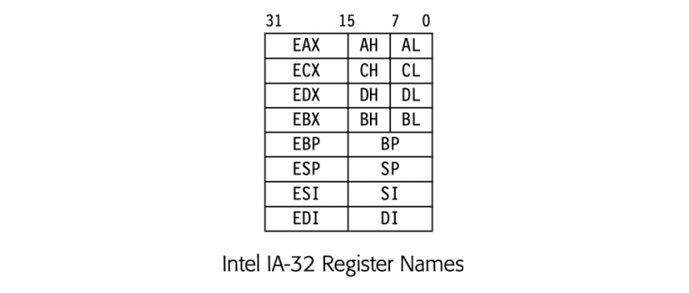
The Intel IA-32 has a small register set, part of which is depicted in Fig. 13.2(b). It provides eight 32-bit registers. The CISC instruction set uses distinct registers for specific purposes, leading to unique names for each register, as shown. For backward compatibility with earlier 16-bit processors, the PR set supports naming subfields of the 32-bit registers.

• In four of the registers, the programmer can name the 32-bit register, its lower 16 bits, and two 8-bit fields. These registers are the accumulator (EAX), the count register (ECX), the data register (EDX), and the base register (EBX).
• In the other four registers, the programmer can name both the 32-bit register and its lower 16 bits. These registers are the base of stack (EBP), the stack pointer (ESP), the string source index pointer (ESI), and the string destination index pointer (EDI).

The figure omits the instruction pointer (EIP and IP) and flag register (FFLAGS and FLAGS), which have both 32-bit and 16-names. The later IA-64 features a larger set of 32-bit GPRs, but preserves the IA-32 names and features in the low numbered registers. Many earlier ISAs used pairing schemes in the FPR set. The drawing in the margin shows how a four register set might work. It would consist of the four 32-bit PRs, F0, F1, F2, and F3. 64-bit values occupy a pair of adjacent registers. If a register pair can begin with any register, then four pairs are possible: D0, D1, D2, and D3.

Some ISAs restrict a register-pair to begin with an odd-numbered register--an aligned pair. With aligned pairs, only the registers shown as D0 and D2 would be available. With aligned pairs, use of D0 precludes the use of F0 and F1. With unaligned pairs, use of D0 still precludes the use of F0 and F1. It also precludes the use of D1 and D3.

In general, the register allocator should make effective use of all available registers. Thus, it must understand the processor's register classes and include mechanisms to use them in a fair and efficient manner. For physically disjoint classes, such as floating-point and general purpose register classes, the allocator can simply allocate them independently. If floating-point spills use GPRs for address calculations, the compiler should allocate the GPRs first.

The design of the register-set name space affects the difficulty of managing register classes in the allocator. For example, the ARM A-64 naming scheme allows the allocator to treat all of the fields in a single PR as a single resource; it can use one of X0 or W0. By contrast, the IA-32 allows concurrent use of both Ah and AL. Thus, the allocator needs more complex mechanisms to handle the IA-32 register set. Section 13.4.7 explores how to build such mechanisms into a global graph-coloring register allocator.

Section review

The register allocator must decide, at each point in the code, which values should be kept in registers. To do so, it computes a name space for the values in the code, often called live ranges. The allocator must discover which live ranges cannot share a register--that is, which live ranges interfere with each other. Finally, it must assign some live ranges to registers and relegate some to memory. It must insert appropriate loads and stores to move values between registers and memory to enforce its decisions.

Review questions

1. Consider a block of straight-line code where the largest register pressure at an operation in the block is $j$. Assume that the allocator is allowed to use $k$ registers. If $j=k$, can the allocator map the live ranges onto the PRs without spilling?
2. Consider a procedure represented as $n$ ILOC operations. Can you bound the number of nodes and edges in the interference graph?

13.3 Local Register Allocation

Recall that a basic block is a maximal length sequence of straight-line code.

The simplest formulation of the register allocation problem is local allocation: consider a single basic block and a single class of $k$ PRs. This problem captures many of the complexities of allocation and serves as a useful introduction to the concepts and terminology needed to discuss global allocation. To simplify the discussion, we will assume that one block constitutes the entire program.

The input code uses source registers, written in code as $s{r}_i$. The output code uses physical registers, written in code as either $p{r}_i$ or simply $r_i$. The physical registers correspond, in general, to named registers in the target ISA.

The input block contains a series of three-address operations, each of which has the form ${\text{op}}_1{\text{ sr}}_1,{\text{ sr}}_2\Rightarrow {\text{ sr}}_n$. From a high-level view, the local register allocator rewrites the block to replace each reference to a source register (SR) with a reference to a specific physical register (PR). The allocator must preserve the input block's original meaning while it fits the computation into the $k$ PRs provided by the target machine.

If, at any point in the block, the computation has more than $k$ live values--that is, values that may be used in the future-then some of those values will need to reside in memory for some portion of their lifetimes. ($k$ registers can hold at most $k$ values.) Thus, the allocator must insert code into the block to move values between memory and registers as needed to ensure that all values are in PRs when needed and that no point in the code needs more than $k$ PRs.

This section presents a version of Best's algorithm, which dates back to the original Fortran compiler. It is one of the strongest known local allocation algorithms. It makes two passes over the code. The first pass derives detailed knowledge about the definitions and uses of values; essentially, it computes Live information within the block. The second pass then performs the actual allocation.

Spill When the allocator moves a live value from a PR to memory, it spills the value.

Restore When the allocator retrieves a previously spilled value from memory, it restores the value.

Best's algorithm has one guiding principle: when the allocator needs a PR and they are all occupied, it should spill the PR that contains the value whose next use is farthest in the future. The intuition is clear; the algorithm chooses the PR that will reduce demand for PRs over the longest interval. If all values have the same cost to spill and restore, this choice is optimal. In practice, that assumption is rarely true, but Best's algorithm still does quite well.

To explain the algorithm it helps to have a concrete data structure. Assume a three-address, ILOC-like code, represented as a list of operations. Each operation, such as $\text{mult}{\text{ sr}}_1,{\text{ sr}}_2\Rightarrow {\text{ sr}}_3$ is represented with a structure:

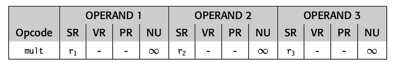
The operation has an opcode, two inputs (operands 1 and 2), and a result (operand 3). Each operand has a source-register name (SR), a virtual-register name (VR), a physical-register name (PR), and the index of its next use (NU).

Register allocation is, at its core, the process of constructing a new name space and modifying the code to use that space. Keeping the SR, VR, and PR names separate simplifies both writing and debugging the allocator.

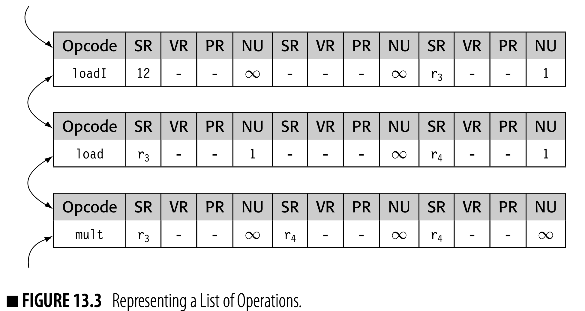
A list of operations might be represented as a doubly linked list, as shown in Fig. 13.3. The local allocator will need to traverse the list in both directions. The list could be created in an array of structure elements, or with individually allocated or block-allocated structures.

Since the meaning is clear, we store a loadI’s constant in its first operand’s SR field.

The first operation, a load1, has an immediate value as its first argument, stored in the SR field. It has no second argument. The next operation, a load, also has just one argument. The final operation, a mult, has two arguments. Because the code fragment does not contain a next use for any of the registers mentioned in the mult operation, their NU fields are set to $\infty$.

13.3.1 Renaming in the Local Allocator

To simplify the local allocator's implementation, the compiler can first rename SRs so that they correspond to live ranges. In a single block, an LR consists of a single definition and one or more uses. The span of the LR is the interval in the block between its definition and its last use.

The renaming algorithm finds the live range of each value in a block. It assigns each LR a new name, its VR name. Finally, it rewrites the code in terms of VRs. Renaming creates a one-to-one correspondence between LRs and VRs which, in turn, simplifies many of the data structures in the local allocator. The allocator then reasons about VRs, rather than arbitrary SR names.

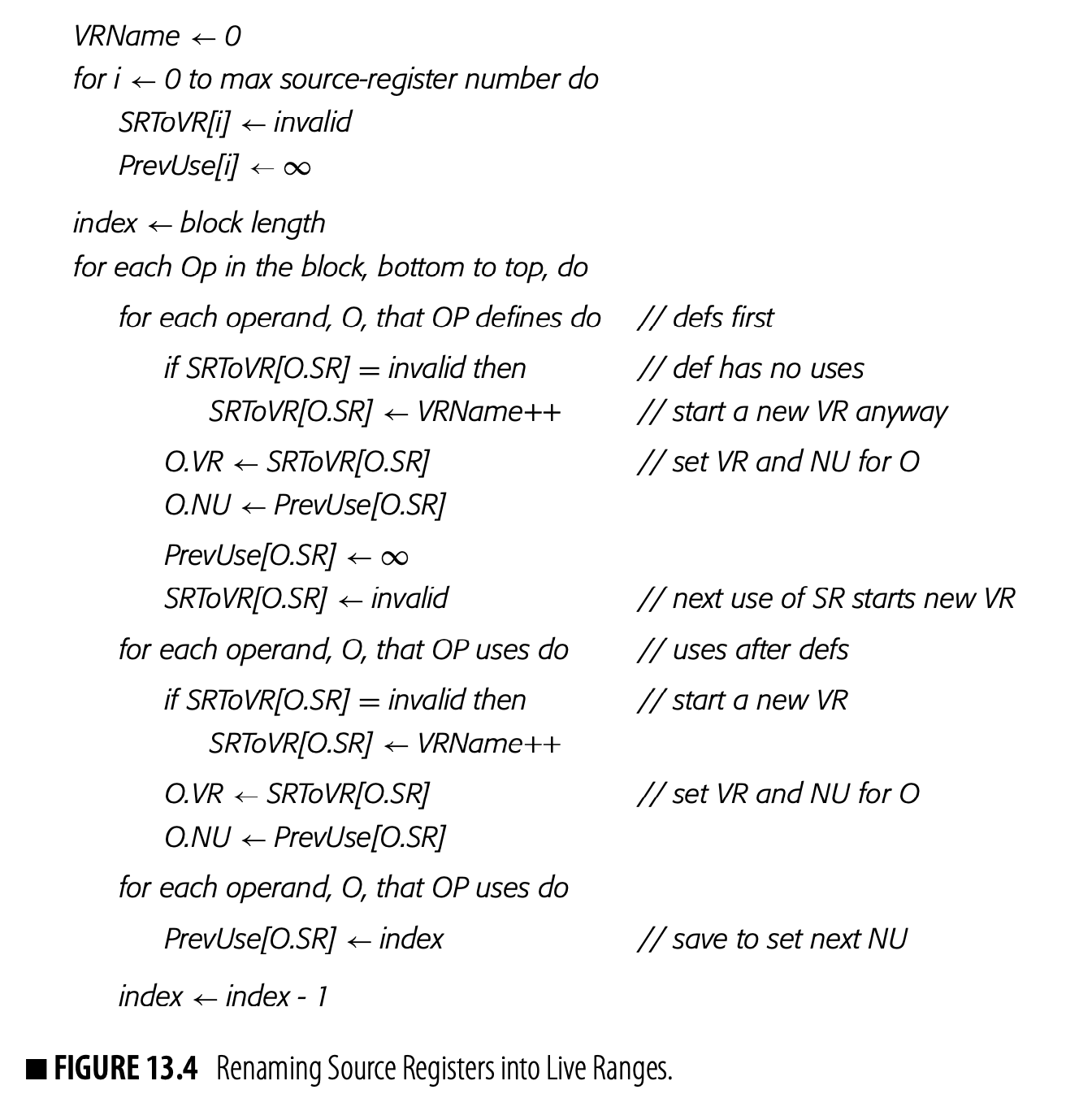
The compiler can discover live ranges and rename them into VRs in a single backward pass over the block. As it does so, it can also collect and record next use information for each definition and use in the block. The algorithm, shown in Fig. 13.4, assumes the representation described in the previous section.

The renaming algorithm builds two maps: SRToVR, which maps an SR name to a VR name, and PreUse, which maps an SR name into the ordinal number of its most recent use. The algorithm begins by initializing each SRToVR entry to invalid and each PrevUse entry to $\infty$.

The algorithm walks the block from the last operation to the first operation. At each operation, it visits definitions first and then uses. At each operand, it updates the maps and defines the VR and NU fields.

If the SR for a definition has no VR, that value is never used. The algorithm still assigns a VR to the SR.

When the algorithm visits a use or def, it first checks whether or not the reference's SR, O.SR, already has a VR. If not, it assigns the next available VR name to the SR and records that fact in SRToVR[O.SR]. Next, it records the VR name and next use information in the operand's record. If the operand is a use, it sets PrevUse[O.SR] to the current operation's index. For a definition, it sets PrevUse[O.SR] back to \infty.

Note that all operands to a store are uses. The store defines a memory location, not a register.

The algorithm visits definitions before uses to ensure that the maps are updated correctly in cases where an SR name appears as both a definition and a use. For example, in add $r_{17},r_{18}\Rightarrow r_{18}$, the algorithm will rewrite the definition with $SRToVR\left[r_{18}\right]$; update $SRToVR\left[r_{18}\right]$ with a new VR name for the use; and then set $PrevUse\left[r_{18}\right]$ to $\infty$.

After renaming, we use live range and virtual register interchangeably.

After renaming, each live range has a unique VR name. An SR name that is defined in multiple places is rewritten as multiple distinct VRs. In addition, each operand in the block has its NU field set to either the ordinal number of the next operation in the block that uses its value, or $\infty$ if it has no next use. The allocator uses this information when it chooses which VRs to spill.

Consider, again, the code from Fig. 13.1. $Panel(a)$ shows the original code. $Panel(b)$ shows that code after renaming. $Panel(c)$ shows the span of each live range, as an interval graph. The allocator does not rename $r_{arp}$ because it is a dedicated PR that holds the activation record pointer and, thus, not under the allocator's control.

MAXLIVE The maximum number of concurrently live VRs in a block

The maximum demand for registers, MAXLIVE, occurs at the start of the first mult operation, marked in panel (c) by the dashed gray line. Six VRs are live at that point. Both ${\mathrm{VR}}_7$ and ${\mathrm{VR}}_8$ are live at the start of the operation. The operation is the last use of ${\mathrm{VR}}_7$ and ${\mathrm{VR}}_8$, as well as the definition of ${\mathrm{VR}}_5$.

13.3.2 Allocation and Assignment

The algorithm for the local allocator appears in Fig. 13.5. It performs allocation and assignment in a single forward pass over the block. It starts with an assumption that no values are in PRs. It iterates through the operations, in order, and incrementally allocates a PR to each VR. At each operation, the allocator performs three steps.

1. To ensure that a use has a PR, the allocator first looks for a PR in the VR-ToPR map. If the entry for VR is invalid, the algorithm calls GetAPR to find a PR. The allocator uses a simple marking scheme to avoid allocating the same PR to conflicting uses in a single operation.

If a single instruction contains multiple operations, the allocator should process all of the uses before any of the definitions.

2. In the second step, the allocator determines if any of the uses are the last use of the VR. If so, it can free the PR, which makes the PR available for reassignment, either to a result of the current operation or to some VR in a future operation.
3. In the third step, the allocator ensures that each VR defined by the operation has a PR allocated to hold its value. Again, the allocator uses GetAPR to find a suitable register.

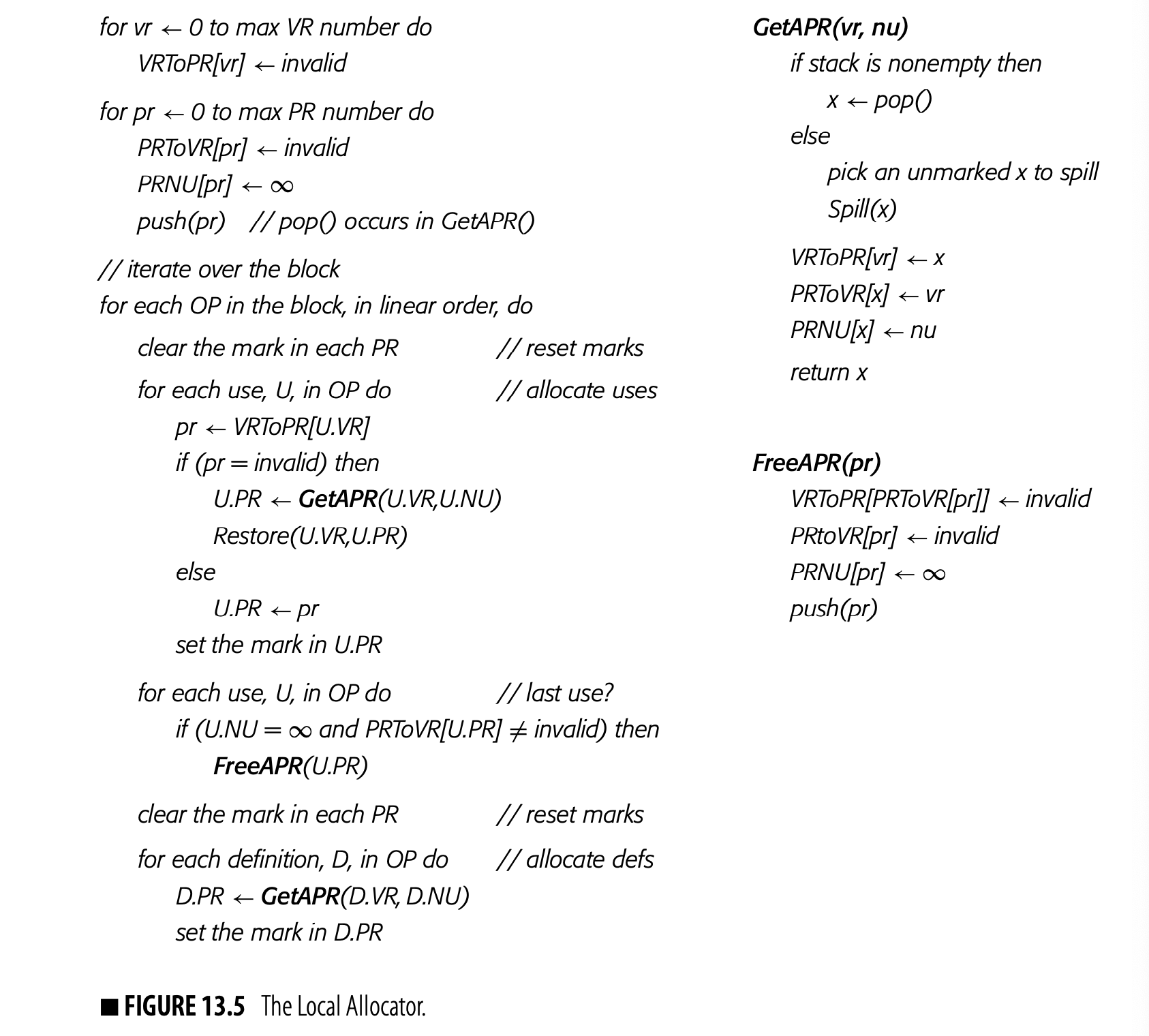
Each of these steps is straightforward, except for picking the value to spill. Most of the complexity of local allocation falls in that task.

The Workings of GetAPR

As it processes an operation, the allocator will need to find a PR for any VR $\nu$ that does not currently have one. This act is the essential act of register allocation. Two situations arise:

1. Some PR $p$ is free: The allocator can assign $p$ to $\nu$. The algorithm maintains a stack of free Prs for efficiency.
2. No PR is free: The allocator must choose a VR to evict from its PR $p$, save the value in $p$ to its spill location, and assign $p$ to hold $\nu$.

If the reference to $\nu$ is a use, the allocator must then restore $\nu$'s value from its memory location to $p$.

SPILL AND RESTORE CODE

At the point where the allocator inserts spill code, all of the physical registers (PRs) are in use. The compiler writer must ensure that the allocator can still spill a value.

Two scenarios are possible. Most likely, the target machine's ISA supports an address mode that allows the spill without need for an additional PR. For example, if the ARP has a dedicated register, say $r_{\text{arp }}$, and the ISA includes an address-immediate store operation, like ILOC's storeAI, then spill locations in the local data area can be reached without an additional PR.

On a target machine that only supports a simple load and store, or an implementation where spill locations cannot reside in the activation record, the compiler would need to reserve a PR for the address computation, reducing the pool of available PRs. Of course, the reserved register is only needed if $MAXLIVE>k$. (If $MAXLIVE\le k$, then no spills are needed and neither is the reserved register.)

Best's heuristic states that the allocator should spill the PR whose current VR has the farthest next use. The algorithm maintains PRNU to facilitate this decision. It simply chooses the PR with the largest PRNU. If the allocator finds two PRs with the same PRNU, it must choose one.

The implementation of PRNU is a tradeoff between the efficiency of updates and the efficiency of searches. The algorithm updates PRNU at each register reference. It searches PRNU at each spill. As shown, PRNU is a simple array; if updates are much more frequent than spills, that makes sense. If spills are frequent enough, a priority queue for PRNU may improve allocation time.

Tracking Physical and Virtual Registers

To track the relationship between VRs and Prs, the allocator maintains two maps. VRToPR contains, for each VR, either the name of the PR to which it is currently assigned, or the value invalid. PRToVR contains, for each PR, either the name of the VR to which it is currently assigned, or the value invalid.

As it proceeds through the block, the allocator updates these two maps so that the following invariant always holds: The code in GetAPR and FreeAPR maintains these maps to ensure that the invariant holds true. In addition, these two routines maintain PRNU, which maps a PR into the ordinal number of the operation where it is next used-a proxy for distance to that next use.

Spills and Restores

Conceptually, the implementation of Spill and Restore from Fig. 13.5 can be quite simple.

Spill locations typically are placed at the end of the local data area in the activation record.

• To spill a PR p, the allocator can use PRToVR to find the VR $v$ that currently lives in p. If v does not yet have a spill location, the allocator assigns it one. Next, it emits an operation to store $p$ into the spill location. Finally, it updates the maps: VRTOPR, PRTOVR, and PRNU.
• To restore a VR v into a PR p, the allocator simply generates a load from v 's spill location into p. As the final step, it updates the maps: VRToPR, PRTOVR, and PRNU.

If all spills have the same cost and all restores have the same cost, then Best's algorithm generates an optimal allocation for a block.

Complications from Spill Costs

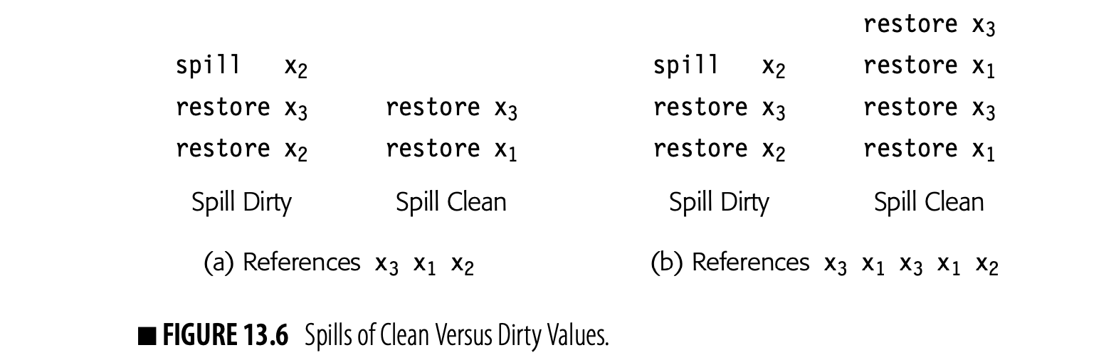
In real programs, spill and restore costs are not uniform. Real code contains both clean and dirty values; the cost to spill a dirty value is greater than the cost to spill a clean value. To see this, consider running the local allocator on a block that contains references to three names, x_{1}, x_{2}, and x_{3}, with just two PRs (k=2).

Assume that the register allocator is at a point where x_{1} and x_{2} are currently in registers and x_{1} is clean and x_{2} is dirty. Fig. 13.6 shows how different spill choices affect the code in two different scenarios.

Reference string A reference string is just a list of references to registers or addresses. In this context, each reference is a use, not a definition.

Panel (a) considers the case when the reference string for the rest of the block is $x_3{x}_1{x}_2$. If the allocator consistently spills clean values before dirty values, it introduces less spill code for this reference string.

Panel (b) considers the case when the reference string for the rest of the block is $x_3{x}_1{x}_3{x}_1{x}_2$. Here, if the allocator consistently spills clean values before dirty values, it introduces more spill code.

The presence of both clean and dirty values fundamentally changes the lo- cal allocation problem. Once the allocator faces two kinds of values with different spill costs, the problem becomes NP-hard. The introduction of re- materializable values, which makes restore costs nonuniform, makes the problem even more complex. Thus, a fast deterministic allocator cannot always make optimal spill decisions. However, these local allocators can produce good allocations by choosing among LRs with different spill costs with relatively simple heuristics.

Remember, however, that the problem is NP-hard. No efficient, deterministic algo- rithm will always produce optimal results.

In practice, the allocator may produce better allocations if it differentiates between dirty, clean, and rematerializable values (see Section 13.2.3). If two PRs have the same distance to their next uses and different spill costs, then the allocator should spill the lower-cost PR.

The issue becomes more complex, however, in choosing between PRs with different spill costs that have next-use distances that are close but not iden- tical. For example, given a dirty value with next use of n and a rematerial- izable value with next use of $n-1$, the latter value will sometimes be the better choice.

Section Review

The limited context in local register allocation simplifies the problem enough so that a fast, intuitive algorithm can produce high-quality allocations. The local allocator described in this section operates on a simple principle: when a PR is needed, spill the PR whose next use is farthest in the future.

In a block where all values had the same spill costs, the local allocator would achieve optimal results. When the allocator must contend with both dirty and clean values, the problem becomes combinatorially hard. A local allocator can produce good results, but it cannot guarantee optimal results.

Review Questions

1. Modify the renaming algorithm, shown in Fig. 13.4, so that is also computes maxlive, the maximum number of simultaneously live values at any instruction in the block.
2. Rematerializing a known constant is an easy decision, because the spill requires no code and the restore is a single load immediate operation. Under what conditions could the allocator profitably rematerialize an operation such as add $r_a,r_b\Rightarrow r_x$?

13.4 Global Allocation via Coloring

Most compilers use a global register allocator--one that considers the entire procedure as context. The global allocator must account for more complex control flow than does a local allocator. Live ranges have multiple definitions and uses; they form complex webs across the control-flow graph. Different blocks execute different numbers of times, which complicates spill cost estimation. While some of the intuitions from local allocation carry forward, the algorithms for global allocation are much more involved.

Spilling an LR breaks it into small pieces that can be kept in distinct PRs.

A global allocator faces another complication: it must coordinate register use across blocks. In the local algorithm, the mapping from an enregistered LR to a PR is, essentially, arbitrary. By contrast, a global allocator must either keep an LR in the same register across all of the blocks where it is live or insert code to move it between registers.

Most global allocation schemes build on a single paradigm. They represent conflicts between register uses with an interference graph and then color that graph to find an allocation. Within this model, the compiler writer faces a number of choices. Live ranges may be shorter or longer. The graph may be precise or approximate. When the allocator must spill, it can spill that lr everywhere or it can spill the lr only in regions of high register pressure.

These choices create a variety of different specific algorithms. This section focuses on one specific set of choices: maximal length live ranges, a precise interference graph, and a spill-everywhere discipline. These choices define the global coloring allocator. Section 13.5 explores variations and improvements to the global coloring allocator.

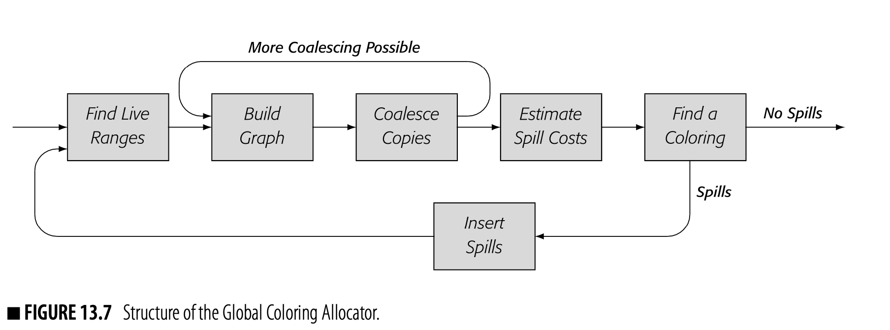
Fig. 13.7 shows the structure of the global coloring allocator.

Find Live Ranges The allocator finds live ranges and rewrites the code with a unique name for each lr. The new name space ensures that distinct values are not constrained simply because they shared the same name in the input code.

Build Graph The allocator builds the interference graph. It creates a node for each lr and adds edges from $L{R}_{\mathrm{i}}$ to any $L{R}_{\mathrm{j}}$ that is live at an operation that defines $L{R}_{\mathrm{i}}$, unless the operation is a copy. Building the graph tends to dominate the cost of allocation.

Coalesce Copies The allocator looks at each copy operation, $L{R}_{\mathrm{i}}\Rightarrow L{R}_{\mathrm{j}}$. If $L{R}_{\mathrm{i}}$ and $L{R}_{\mathrm{j}}$ do not interfere, it combines the lRs, removes the copy, and updates the graph. Coalescing reduces the number of lRs and reduces the degree of other nodes in the graph.

Unfortunately, the graph update is conservative rather than precise (see Section 13.4.3). Thus, if any LRs are combined, the allocator iterates the Build-Coolesce process until it cannot coalesce any more LRs--typically two to four iterations.

The spill cost computation has many corner cases (see Sections 13.2.3 and 13.4.4).

Estimate Spill Costs: The allocator computes, for each lr, an estimate of the runtime cost of spilling the entire lr. It adds the costs of the spills and restores, each multiplied by the estimated execution frequency of the block where the code would be inserted.

Find a Coloring: The allocator tries to construct a $k$-coloring for the interference graph. It uses a two-phase process: graph simplification to construct an order for coloring, then graph reconstruction that assigns colors as it reinserts each node back into the graph.

If the allocator finds a $k$-coloring, it rewrites the code and exits. If any nodes remain uncolored, the allocator invokes Insert Spills to spill the uncolored LRs. It then restarts the allocator on the modified code.

The second and subsequent attempts at coloring take less time than the first try because coalescing in the first pass has reduced the size of both the problem and the interference graph.

Insert Spills: For each uncolored lr, the allocator inserts a spill after each definition and a restore before each use. This converts the uncolored lr into a set of tiny LRs, one at each reference. This modified program is easier to color than the original code.

The following subsections describe these phases in more detail.

13.4.1 Find Global Live Ranges

GRAPH COLORING

Graph coloring is a common paradigm for global register allocation. For an arbitrary graph G, a coloring of G assigns a color to each node in G so that no pair of adjacent nodes has the same color. A coloring that uses k colors is termed a k-coloring, and the smallest such k for a given graph is called the graph’s minimum chromatic number. Consider the following graphs: The graph on the left is two-colorable. For example, we can assign blue to nodes 1 and 5 , and red to nodes 2,3 , and 4 . Adding the edge (2,3), as shown on the right, makes the graph three-colorable, but not two-colorable. (Assign blue to nodes 1 and 5 , red to nodes 2 and 4 , and yellow to node 3 .)

For a given graph, finding its minimum chromatic number is NP-complete. Similarly, determining if a graph is k-colorable, for fixed k, is NP-complete. Graph coloring allocators use approximate methods to find colorings that fit the available resources.

The maximum degree of any node in a graph gives an upper bound on the graph's chromatic number. A graph with maximum degree of $x$ can always be colored with $x+1$ colors. The two graphs shown above demonstrate that degree is a loose upper bound. Both graphs have maximum degree of three. Both graphs have colorings with fewer than four colors. In each case, high-degree nodes have neighbors that can receive the same color.

As its first step, the global allocator constructs maximal-sized global live ranges (see Section 13.2.1). A global lr is a set of definitions and uses that contains all of the uses that a definition in the set can reach, along with all of the definitions that can reach those uses. Thus, the LR forms a complex web of definitions and uses that, ideally, should reside in a single PR.

The algorithm to construct live ranges is straightforward if the allocator can work from the SSA form of the code. Thus, the first step in finding live ranges is to convert the input code to SSA form, if necessary. The allocator can then build maximal-sized live ranges with a simple approach: at each $\varphi$-function, combine all of the names, both definition and uses, into a single LR. If the allocator applies this rule at each $\varphi$-function, it creates the set of maximal global LRs.

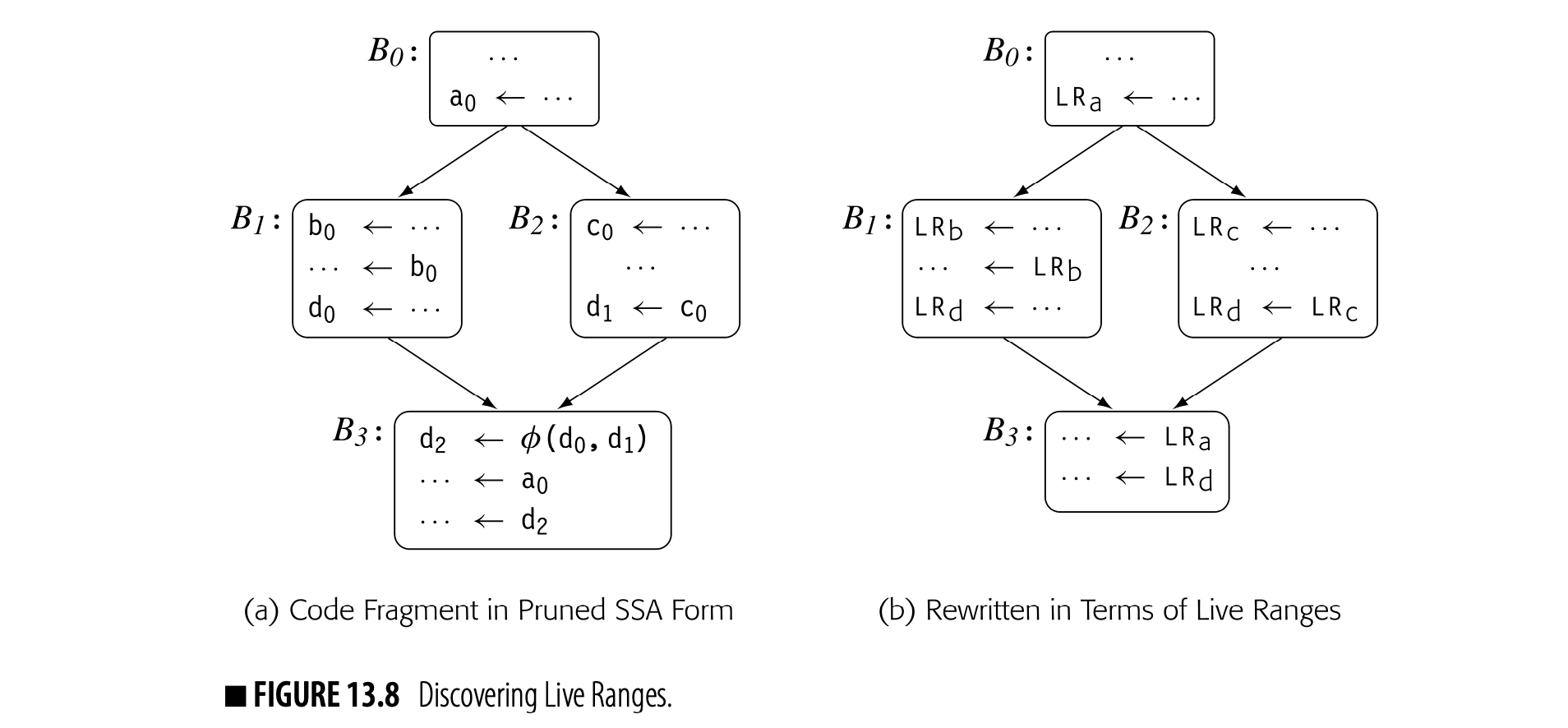
To make this process efficient, the compiler can use the disjoint-set union-find algorithm. To start, it assigns a unique set name to each SSA name. Next, it visits each $\varphi$-function in the code and unions together the sets associated with each $\varphi$-function parameter and the set for the $\varphi$-function result. After all of the $\varphi$-functions have been processed, each remaining unique set becomes an LR. The allocator can either rewrite the code to use LR names or it can create and maintain a mapping between SSA names and LR names. In practice, the former approach seems simpler.

Since the process of finding LRs does not move any definitions or uses, translation out of SSA form is trivial. The LR name space captures the effects that would require new copies during out-of-SSA translation. Thus, the compiler can simply drop the $\varphi$-functions and SSA-names during renaming.

Fig. 13.8(a) shows a code fragment in semiprunned SSA form that involves source-code variables, a, b, c, and d. To find the live ranges, the allocator assigns each SSA name a set that contains its name. It unions together the sets associated with names used in the $\varphi$-function, $\{{\text{d}}_{\text{0}}\}\cup \{{\text{d}}_{\text{1}}\}\cup \{{\text{d}}_{\text{2}}\}$. This gives a final set of four LRs: ${\text{LR}}_{\text{a}}=\{{\text{a}}_{\text{0}}\}$, ${\text{LR}}_{\text{b}}=\{{\text{b}}_{\text{0}}\}$, ${\text{LR}}_{\text{c}}=\{{\text{c}}_{\text{0}}\}$, and ${\text{LR}}_{\text{d}}=\{{\text{d}}_{\text{0}},{\text{d}}_{\text{1}},{\text{d}}_{\text{2}}\}$. Fig. 13.8(b) shows the code rewritten to use the LRs.

13.4.2 Build an Interference Graph

To model interferences, the global allocator builds an interference graph, $I=(N,E)$. Nodes in $N$ represent individual live ranges and edges in $E$ represent interferences between live ranges. Thus, an undirected edge $(n_i,n_j)\in E$ exists if and only if the corresponding live ranges ${\text{LR}}_{\text{i}}$ and ${\text{LR}}_{\text{j}}$ interfere. The interference graph for the code in Fig. 13.8(b) appears in the margin.

$\mathrm{L}{\mathrm{R}}_{\mathrm{a}}$ interferes with each of $\mathrm{L}{\mathrm{R}}_{\mathrm{b}}$, $\mathrm{L}{\mathrm{R}}_{\mathrm{c}}$, and $\mathrm{L}{\mathrm{R}}_{\mathrm{d}}$. None of $\mathrm{L}{\mathrm{R}}_{\mathrm{b}}$, $\mathrm{L}{\mathrm{R}}_{\mathrm{c}}$, or $\mathrm{L}{\mathrm{R}}_{\mathrm{d}}$ interfere with each other; they could share a single $\mathrm{PR}$.

If the compiler can color $I$ with $k$ or fewer colors, then it can map the colors directly onto $\mathrm{PR}$s to produce a legal allocation. In the example, $\mathrm{L}{\mathrm{R}}_{\mathrm{a}}$ interferes with each of $\mathrm{L}{\mathrm{R}}_{\mathrm{b}}$, $\mathrm{L}{\mathrm{R}}_{\mathrm{c}}$, and $\mathrm{L}{\mathrm{R}}_{\mathrm{d}}$. In a coloring, $\mathrm{L}{\mathrm{R}}_{\mathrm{a}}$ must receive its own color and, in an allocation, it cannot share a $\mathrm{PR}$ with $\mathrm{L}{\mathrm{R}}_{\mathrm{b}}$, $\mathrm{L}{\mathrm{R}}_{\mathrm{c}}$, or $\mathrm{L}{\mathrm{R}}_{\mathrm{d}}$. The other live ranges do not interfere with each other. Thus, $\mathrm{L}{\mathrm{R}}_{\mathrm{b}}$, $\mathrm{L}{\mathrm{R}}_{\mathrm{c}}$, and $\mathrm{L}{\mathrm{R}}_{\mathrm{d}}$ could share a single $\mathrm{color}$ and, in the code, a single $\mathrm{PR}$. This interference graph is two-colorable, and the code can be rewritten to use just two registers. Now, consider what would happen if another phase of the compiler reordered the last two definitions in $B_I$, as shown in the margin. This change makes $\mathrm{L}{\mathrm{R}}_{\mathrm{b}}$ live at the definition of $\mathrm{L}{\mathrm{R}}_{\mathrm{d}}$. It adds an edge ($\mathrm{L}{\mathrm{R}}_{\mathrm{b}}$,$\mathrm{L}{\mathrm{R}}_{\mathrm{d}}$) to the interference graph, which makes the graph three-colorable rather than two-colorable. (The graph is small enough to prove this by enumeration.) With this new graph, the allocator has two options: to use three registers, or, if only two registers are available, to spill one of $\mathrm{L}{\mathrm{R}}_{\mathrm{b}}$ or $\mathrm{L}{\mathrm{R}}_{\mathrm{a}}$ before the definition of $\mathrm{L}{\mathrm{R}}_{\mathrm{d}}$ in $B_I$. Alternatively, the allocator could reorder the two operations and eliminate the interference between $\mathrm{L}{\mathrm{R}}_{\mathrm{b}}$ and $\mathrm{L}{\mathrm{R}}_{\mathrm{d}}$. Typically, register allocators do not reorder operations. Instead, allocators assume a fixed order of operations and leave ordering questions to the instruction scheduler (see Chapter 12).

Section 11.3.2 also uses LIVENOW.

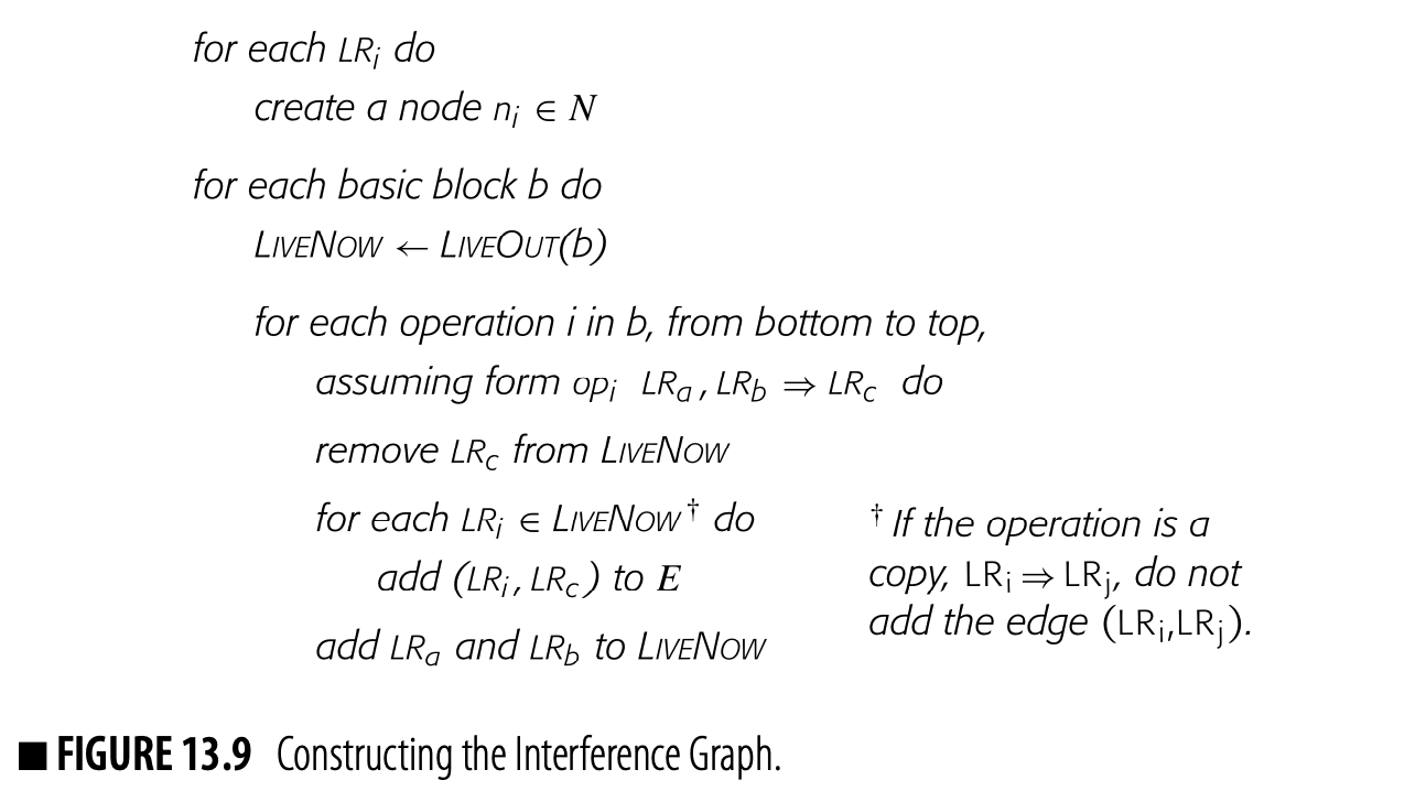
Given the code, renamed into $\mathrm{LR}$s, and $\mathrm{LiveOut}$ sets for each block in the renamed code, the allocator can build the interference graph in one pass over each block, as shown in Fig. 13.9. The algorithm walks the block, from bottom to top. At each operation, it computes $\mathrm{LiveNow}$, the set of values that are live at the current operation. At the bottom of the block, $\mathrm{LiveOut}$ and $\mathrm{LiveNow}$ must be identical. As the algorithm walks backward through the block, it adds the appropriate interference edges to the graph and updates the LiveNow set to reflect each operation's impact.

The algorithm implements the definition of interference given earlier: $L{R}_{\mathrm{i}}$ and $L{R}_{\mathrm{j}}$ interfere only if $L{R}_{\mathrm{i}}$ is live at a definition of $L{R}_{\mathrm{j}}$, or vice versa. The allocator adds, at each operation, an interference between the defined $LR$ and each $LR$ that is live after the operation.

Copy operations require special treatment. A copy $L{R}_{\mathrm{i}}\Rightarrow L{R}_{\mathrm{j}}$ does not create an interference between $L{R}_{\mathrm{i}}$ and $L{R}_{\mathrm{j}}$ because the two live ranges have the same value after the copy executes and, thus, could occupy the same register. If subsequent context creates an interference between these live ranges, that operation will create the edge. Treating copies in this way creates an interference graph that precisely captures when $L{R}_{\mathrm{i}}$ and $L{R}_{\mathrm{j}}$ can occupy the same register. As the allocator encounters copies, it should create a list of all the copy operations for later use in coalescing.

Insertion into the lists should check the bit-matrix to avoid duplication.

To improve the allocator's efficiency, it should build both a lower-triangular bit matrix and a set of adjacency lists to represent $E$. The bit matrix allows a constant-time test for interference, while the adjacency lists allow efficient iteration over a node's neighbors. The two-representation strategy uses more space than a single representation would, but pays off in reduced allocation time. As suggested in Section 13.2.4, the allocator can build separate graphs for disjoint register classes, which reduces the maximum graph size.

13.4.3 Coalesce Copy Operations

The allocator can use the interference graph to implement a strong form of copy coalescing. If the code contains a copy operation, $L{R}_{\mathrm{i}}\Rightarrow L{R}_{\mathrm{j}}$, and the allocator can determine that $L{R}_{\mathrm{i}}$ and $L{R}_{\mathrm{j}}$ do not interfere at some other operation, then the allocator can combine the $L{R}_{\mathrm{s}}$ and remove the copy operation. We say that the copy has been "coalesced."

In his thesis, Briggs shows examples where coalescing eliminates up to one-third of the initial live ranges.

Coalescing a copy has several beneficial effects. It eliminates the actual copy operation, which makes the code smaller and, potentially, faster. It reduces the degree of any $LR$ that previously interfered with both $L{R}_{\mathrm{i}}$ and $L{R}_{\mathrm{j}}$. It removes a node from the graph. Each of these effects makes the coloring pass faster and more effective.

Fig. 13.10 shows a simple, single-block example. The original code appears in panel (a). Intervals to the right indicate the extents of the live ranges that are involved in the copy operation. Even though $L{R}_{\mathrm{a}}$ overlaps both $L{R}_{\mathrm{b}}$ and $L{R}_{\mathrm{c}}$, it interferes with neither of them because the overlaps involve copy operations. Since $L{R}_{\mathrm{b}}$ is live at the definition of $L{R}_{\mathrm{c}}$, $L{R}_{\mathrm{b}}$ and $L{R}_{\mathrm{c}}$ interfere. Both copy operations are candidates for coalescing.

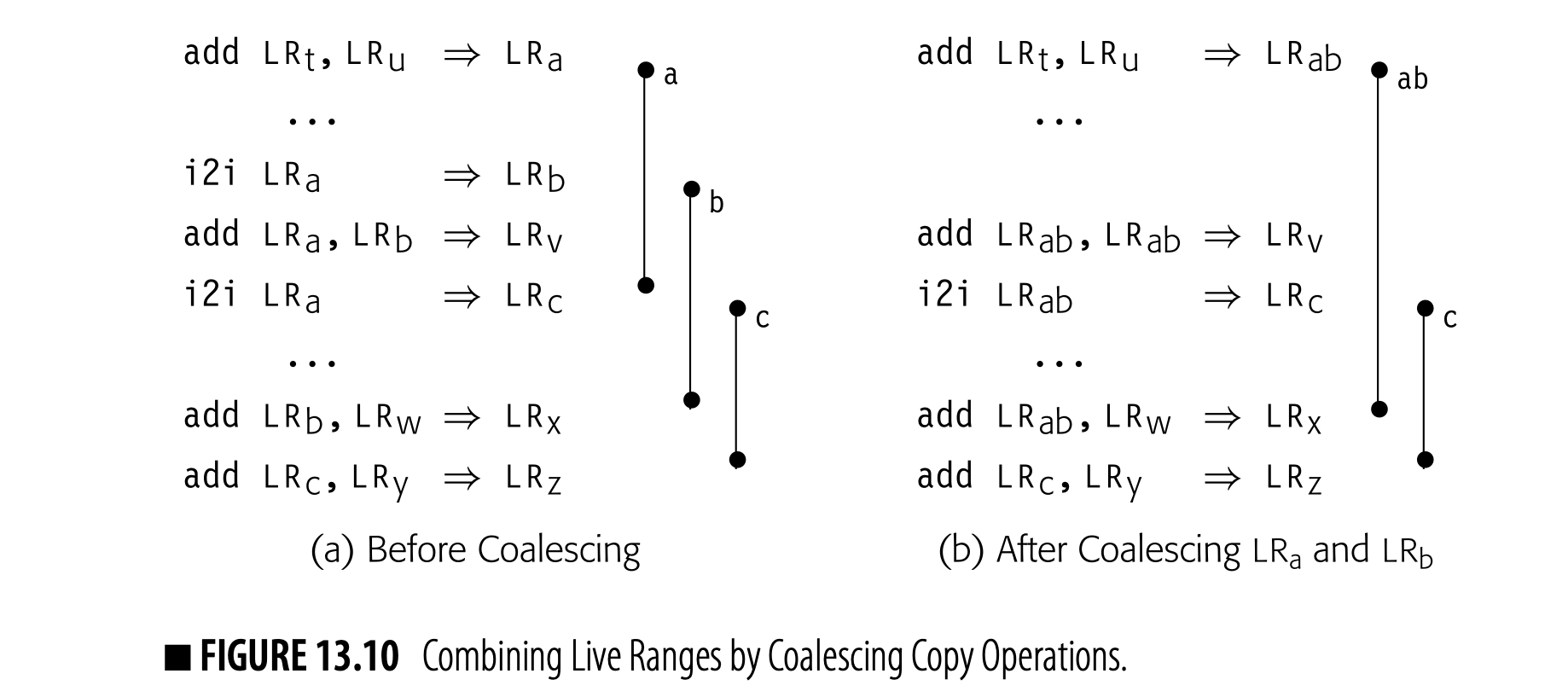
Fig. 13.10(b) shows the result of coalescing LR${}_{\text{a}}$ and LR${}_{\text{b}}$ to produce LR${}_{\text{ab}}$. LR${}_{\text{ab}}$ and LR${}_{\text{c}}$ still do not interfere, because LR${}_{\text{c}}$ is created by the copy operation from LR${}_{\text{ab}}$. Combining LR${}_{\text{a}}$ and LR${}_{\text{b}}$ reduces LR${}_{\text{v}}^{\circ }$ by one. Before coalescing, both LR${}_{\text{a}}$ and LR${}_{\text{b}}$ interfered with LR${}_{\text{v}}$. After coalescing, those values occupy a single LR rather than two LRs. In general, coalescing two live ranges either decreases the degrees of their neighbors or leaves them unchanged; it cannot increase their degrees.

The membership test should use the bit- matrix for efficiency.

To perform coalescing, the allocator walks the list of copies from Build Graph and inspects each operation, LR${}_{\text{i}}\Rightarrow$ LR${}_{\text{j}}$. If $({\text{LR}}_{\text{i}},{\text{LR}}_{\text{j}})\notin E$, then LR${}_{\text{i}}$ and LR${}_{\text{j}}$ do not interfere and the allocator combines them, eliminates the copy, and updates $I$ to reflect the new, combined LR${}_{\text{ij}}$. The allocator can conservatively update $I$ by moving each edge from LR${}_{\text{i}}$ and LR${}_{\text{j}}$ to LR${}_{\text{ij}}$, eliminating duplicates. This update is not precise, but it lets the allocator continue coalescing.

In practice, allocators coalesce every live range that they can, given the interferences in $I$. Then, they rewrite the code to reflect the revised LRs and eliminate the coalesced copies. Next, they rebuild $I$ and try again to coalesce copies. This process typically halts after a couple of rounds of coalescing.

The example illustrates the imprecise nature of this conservative update to the graph. The update moves the edge $({\text{LR}}_{\text{b}},{\text{LR}}_{\text{c}})$ from LR${}_{\text{b}}$ to LR${}_{\text{ab}}$, when, in fact, LR${}_{\text{ab}}$ and LR${}_{\text{c}}$ do not interfere. Rebuilding the graph from the transformed code yields the precise interference graph, without $({\text{LR}}_{\text{ab}},{\text{LR}}_{\text{c}})$. At that point, the allocator can coalesce LR${}_{\text{ab}}$ and LR${}_{\text{c}}$.

If the allocator can coalesce LR${}_{\text{i}}$ with either LR${}_{\text{j}}$ or LR${}_{\text{k}}$, choosing to form LR${}_{\text{ij}}$ may prevent a subsequent coalesce with LR${}_{\text{k}}$, or vice versa. Thus, the order of coalescing matters. In principle, the compiler should coalesce the most frequently executed copies first. Thus, the allocator might coalesce copies in order by the estimated execution frequency of the block that contains the copy. To implement this, the allocator can consider the basic blocks in order from most deeply nested to least deeply nested.

This strategy applies a lesson from semipruned SSA form: only include the names that matter.

In practice, the cost of building the interference graph for the first round of coalescing dominates the overall cost of the graph-coloring allocator. Subsequent passes through the build-coalesce loop process a smaller graph and, therefore, run more quickly. To reduce the cost of coalescing, the compiler can build a subset of the interference graph--one that only includes live ranges involved in a copy operation.

13.4.4 Estimate Global Spill Costs

When a register allocator discovers that it cannot keep all of the live ranges in registers, it must select an lr to spill. Typically, the allocator uses some carefully designed metric to rank the choices and picks the lr that its metric suggests is the best spill candidate. The local allocator used the distance to the lr's next use, which works well in a single-block context. In the global allocator, the metric incorporates an estimate of the runtime costs that will be incurred by spilling and restoring a particular lr.

To compute the estimated spill costs for an lr, the allocator must examine each definition and use in the lr. At each definition, it estimates the cost of a spill after the definition and multiplies that number by the estimated execution frequency of the block that contains the definition. At each use, it estimates the cost of a restore before the use and multiplies that number by the estimated execution frequency of the block that contains the use. It sums together the estimated costs for each definition and use in the lr to produce a single number. This number becomes the spill cost for the lr.

Of course, the actual computation is more complex than the preceding explanation suggests. At a given definition or use of an lr, the value might be any of dirty, clean, or rematerializable (see Section 13.2.3). Individual definitions and uses within an lr can have different classifications, so the allocator must perform enough analysis to classify each reference in the lr. That classification determines the cost to spill or restore that reference.

The precise execution count of a block is difficult to determine. Fortunately, relative execution frequencies are sufficient to guide spill decisions; the allocator needs to know that one reference is likely to execute much more often than another. Thus, the allocator derives, for each block, a number that indicates its relative execution frequency. Those frequencies apply uniformly to each reference in the block.

The allocator could compute spill costs on demand--when it needs to make a spill decision. If it finds a $k$-coloring without any spills, an on-demandcost computation would reduce overall allocation time. If the allocator must spill frequently, a batch cost computation would, most likely, be faster than an on-demand computation.

Fig. 13.7 suggests that the allocator should perform the cost computation before it tries to color the graph. The allocator can defer the computation until the first time that it needs to spill. If the allocator does not need to spill, it avoids the overhead of computing spill costs; if it does spill, it computes spill costs for a smaller set of LRs.

Accounting for Execution Frequencies

Using the 1$0^d$ estimator can introduce a problem with integer overflow in the spill cost computation. Many compiler writers have discovered this issue experimentally. Deeply nested loops may need floating-point spill costs.

To compute spill costs, the allocator needs an estimate of the execution frequency for each basic block. The compiler can derive these estimates from profile data or from heuristics. Many compilers assume that each loop executes 10 times, which creates a weight of $10^d$ for a block nested inside $d$ loops. This assumption assigns a weight of 10 to a block inside one loop, 100 to a block inside two nested loops, and so on. An unpredictable if-then-else would decrease the estimated frequency by half. In practice, these estimates create a large enough bias to encourage spilling LRs in outer loops rather than those in inner loops.

Negative Spill Costs

A live range that contains a load, a store, and no other uses should receive a negative spill cost if the load and store refer to the same address. (Optimization can create such live ranges; for example, if the use were optimized away and the store resulted from a procedure call rather than the definition of a new value.) Sometimes, spilling a live range may eliminate copy operations with a higher cost than the spill operations; such a live range also has a negative cost. Any live range with a negative spill cost should be spilled, since doing so decreases demand for registers and removes operations from the code.

Infinite Spill Costs

Some live ranges are so short that spilling them does not help. Consider the short LR shown in the left margin. If the allocator tries to spill LR, it will insert a store after the definition and a load before the use, creating two new LRs. Neither of these new LRs uses fewer registers than the original LR, so the spill produces no benefit. The allocator should assign the original LR a spill cost of infinity, ensuring that the allocator does not try to spill it. In general, an LR should have infinite spill cost if no other LR ends between its definitions and its uses. This condition stipulates that availability of registers does not change between the definitions and uses.

Infinite-cost live ranges present a code-shape challenge to the compiler. If the code contains more than $k-1$ nested infinite-cost LRs, and no LR ends in this region, then the infinite-cost LRs form an uncolorable clique in the interference graph. While such a situation is unusual, we have seen it arise in practice. The register allocator cannot fix this problem; the compiler writer must simply ensure that the allocator does not receive such code.

13.4.5 Color the Graph

The global allocator colors the graph in a two-step process. The first step, called Simplify, computes an order in which to attempt the coloring. The second step, called Select, considers each node, in order, and tries to assign it a color from its set of $k$ colors.

To color the graph, the allocator relies on a simple observation:

If a node has fewer than $k$ neighbors, then it must receive a color, independent of the colors assigned to its neighbors.

Thus, any node $n$ with degree less than $k$, denoted $n^{\circ }<k$, is trivial to color. The allocator first tries to color those nodes that are hard to color; it defers trivially colored nodes until after the difficult nodes have been colored.

Simplify

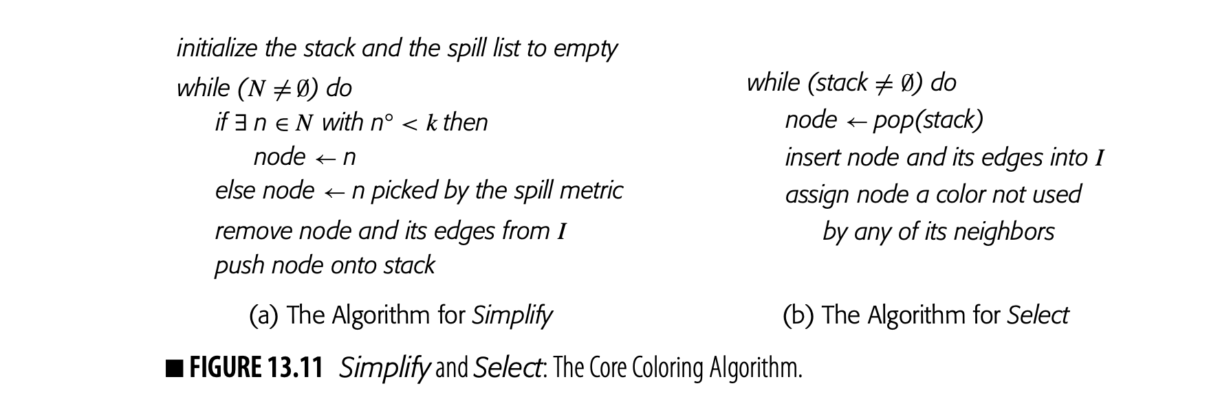
To compute an order for coloring, the allocator finds trivially colored nodes and removes them from the graph. It records the order of removal by pushing the nodes onto a stack as they are removed. The act of removing a node and its edges from the graph lowers the degree of all its neighbors. Fig. 13.11(a) shows the algorithm.

As nodes are removed from the graph, the allocator must preserve both the node and its edges for subsequent reinsertion in Select. The allocator can either build a structure to record them, or it can add a mark to each edge and each node indicating whether or not it is active.

Spill metric a heuristic used to select an LR to spill

Sirplify uses two distinct mechanisms to select the node to remove next. If there exists a node $n$ with $n^{\circ }<k$, the allocator chooses that node. Because these nodes are trivially colored, the order in which they are removed does not matter. If all remaining nodes are constrained, with degree $\ge k$, then the allocator picks a node to remove based on its spill metric. Any node $n$ removed by this process has $n^{\circ }\ge k$; thus, it may not receive a color during the assignment phase. The loop halts when the graph is empty. At that point, the stack contains all the nodes in order of removal.

Select

To color the graph, the allocator rebuilds the interference graph in the reverse of the removal order. It repeatedly pops a node $n$ from the stack, inserts $n$ and its edges back into $I$, and picks a color for $n$ that is distinct from $n$'s neighbors. Fig. 13.11(b) shows the algorithm.

In our experience, the order in which the allocator considers colors has little practical impact.

To select a color for node $n$, the allocator tallies the colors of $n$'s neighbors in the current graph and assigns $n$ an unused color. It can search the set of colors in a consistent order, or it can assign colors in a round-robin fashion. If no color remains for $n$, it is left uncolored.

When the stack is empty, $I$ has been rebuilt. If every node has a color, the allocator rewrites the code, replacing LR names with pr names, and returns. If any nodes remain uncolored, the allocator spills the corresponding LRs. The allocator passes a list of the uncolored LRs to insert Spills, which adds the spills and restores to the code. Insert Spills then restarts the allocator on the revised code. The process repeats until every node in $I$ receives a color. Typically, the allocator finds a coloring and halts in a couple of trips around the large loop in Fig. 13.7.

Why Does This Work?

The global allocator inserts each node back into the graph from which it was removed. If the reduction algorithm removes the node for ${\mathrm{LR}}_n$ from $I$ because $n^{\circ }<k$, then it reinserts ${\mathrm{LR}}_n$ into a graph in which $n^{\circ }<k$ and node $n$ is trivially colored.

The only way that a node $n$ can fail to receive a color is if $n$ was removed from $I$ using the spill metric. Select reinserts such a node into a graph in which $n^{\circ }\ge k$. Notice, however, that this condition is a statement about degree in the graph, rather than a statement about the availability of colors.

If node $n$'s neighbors use all $k$ colors, then the allocator finds no color for $n$. If, instead, they use fewer than $k$ colors, then the allocator finds a color for $n$. In practice, a node $n$ often has multiple neighbors that use the same color. Thus, Select often finds colors for some of these constrained nodes.

Updating the Interference Graph Both coalescing and spilling change the set of nodes and edges in the interference graph. In each case, the graph must be updated before allocation can proceed.

The global coloring allocator uses a conservative update after each coalesce; that update also triggers another iteration around the Build-Coalesce loop in Fig. 13.7.It obtains precision in the graph by rebuilding it from scratch.

The allocator defers spill insertion until the end of the Simplify-Select process; it then inserts all of the spill code and triggers another iteration of the Build-Coalesce-Spill Costs-Color loop. Again, it obtains precision by rebuilding the graph.

If the allocator could update the graph precisely, it could eliminate both of the cycles shown in Fig. 13.7. Coalescing could complete in a single pass. It could insert spill code incrementally when it discovered an uncolored node; the updated graph would correctly reflect interferences for color selection.

Better incremental updates can reduce allocation time. A precise update would produce the same allocation as the original allocator, within variance caused by changes in the order of decisions. An imprecise but conservative update could produce faster allocations, albeit with some potential decrease in code quality from the imprecision in the graph. DasGupta

Simplify determines the order in which Select tries to color nodes. This order plays a critical role in determining which nodes receive colors. For a node $n$ removed from the graph because $n^{\circ }<k$, the order is unimportant with respect to the nodes that remain in the graph. The order may be important with respect to nodes already on the stack; after all, $n$ may have been constrained until some of those earlier nodes were removed. For nodes removed from the graph using the spill metric, the order is crucial. The else clause in Fig. 13.11(a) executes only when every remaining node has degree $\ge k$. Thus, the nodes that remain in the graph at that point are in more heavily connected subgraphs of $I$.

The original global coloring allocator appeared in IBM’s PL.8 compiler.

The order of the constrained nodes is determined by the spill metric. The original coloring allocator picked a node that minimized the ratio of $cost÷degree$, where $cost$ is the estimated spill cost and $degree$ is the node's degree in the current graph. This metric balances between spill cost and the number of nodes whose degree will decrease.

Other spill metrics have been tried. Several metrics are variations on $cost÷degree$, including $cost÷degre{e}^2$, $cost÷area$ and $cost÷are{a}^2$, where the $area$ of an LR is defined as the sum of MAXLIVE taken over all theinstructions that lie within the LR. These metrics try to balance the cost of spilling a specific LR against the extent to which that spill makes it easier to color the rest of the graph. Straight cost has been tried; it focuses on runtime speed. In code-space sensitive applications, a metric of total spill operations can drive down the code-space growth from spilling.

In practice, no single heuristic dominates the others. Since coloring is fast relative to building $I$, the allocator can color $I$ with several different spill metrics and keep the best result.

13.4.6 Insert Spill and Restore Code

The spill code created by a global register allocator is no more complex than the spill code inserted in the local allocator. Insert Spills receives a list of Lrs that did not receive a color. For each LR, it inserts the appropriate code after each definition and before each use.

The same complexities that arose in the local allocator apply in the global case. The allocator should recognize the distinction between dirty values, clean values, and rematerializable values. In practice, it becomes more complex to recognize whether a value is dirty, clean, or rematerializable in the global scope.

The global allocator applies a spill everywhere discipline. An uncolored live range is spilled at every definition point and restored at every use point. In practice, a spilled LR often has definitions and uses that occur in regions where Prs are available. Several authors have looked at techniques to loosen the spill everywhere discipline so as to keep spilled Lrs in Prs in regions of low register pressure (see the discussions in Section 13.5).

13.4.7 Handling Overlapping Register Classes

In practice, the register allocator must deal with the idiosyncratic properties of the target machine's register set and its calling convention. This reality constrains both allocation and assignment.

For example, on the ARM A-64, the four floating-point registers Q1, Q1, S1, and H1 all share space in a single PR, as shown in the margin. Thus, if the compiler allocates Q1 to hold LRi, Q1, S1, and H1 are unavailable while LRi is live. Similar restrictions arise with the overlapped general purpose registers, such as the pair X3 and W3.

To understand how overlapping register classes affect the structure of a register allocator, consider how the local allocator might be modified to handle the ARM A-64 general purpose registers.

The algorithm, as presented, uses one attribute to describe an LR, its virtual register number. With overlapping classes, such as Xi and Wi, each LR also needs an attribute to describe its class.

• The stack of free registers should use names drawn from one of the two sets of names, Xi or Wi. The state, allocated or free, of a coresident pair such as X0 and WO is identical.
• The mappings VRT0PR, PRT0VR, and PRNU can also remain single-valued. If ${VR}_i$ has an allocated register, VRT0PR will map the vr's num field to a register number and its class field will indicate whether to use the X name or the W name.

Because the local algorithm has a simple way of modeling the status of the prs, the extensions are straightforward. To handle a more complex situation, such as the EAX register on the IA-32, the local allocator would need more extensive modifications. Use of EAX requires the entire register and precludes simultaneous use of AH or AL. Similarly, use of either AH or AL precludes simultaneous use of EAX. However, the allocator can use both AL and AH at the same time. Similar idiosyncratic rules apply to the other overlapping names, shown in the margin and in Fig. 13.2(b).

The global graph-coloring allocators have more complex models for interference and register availability than the local allocator. To adapt them for fair use of overlapping register classes requires a more involved approach.

Describing Register Classes

Before we can describe a systematic way to handle allocation and assignment for multiple register classes, we need a systematic way to describe those classes. The compiler can represent the members of each class with a set. From Fig. 13.2(a), the ARM A-64 has six classes:

Thus, $\text{class}(\text{D3})=\{\text{00},\text{01},\dots ,\text{031}\}$, the set of 64-bit floating-point registers.

The simplest scheme to describe overlap between register classes is to introduce a function, $\text{alias}(r)$. For a register name $r$, $\text{alias}(r)$ maps $r$ to the set of register names that occupy physical space that intersects with $r$'s space. In the ARM A-64, $\text{alias}(\text{WI})=\{\text{X1}\}$ and $\text{alias}(\text{S2})=\{\text{02},\text{02},\text{02}\}$. Similarly, in IA-32, $\text{alias}(\text{AH})=\{\text{EA}\}$, $\text{alias}(\text{AL})=\{\text{EA}\}$, and $\text{alias}(\text{EAX})=\{\text{AL},\text{AH}\}$. Because AL and AH occupy disjoint space, they are not aliases of each other.

The compiler can compute the information that it will need for allocation and assignment from the class and alias relationships.

Coloring with Overlapping Classes

The presence of overlapping register classes complicates each of coloring, assignment, and coalescing.

Coloring

The graph-coloring allocator approximates colorability by comparing a node's degree against the number of available colors. If $n^{\circ }<k$, the number of available registers, then Simplify categorizes $n$ as trivially colored, removes $n$ from the graph, and pushes $n$ onto the ordering stack. If the graph contains no trivially colored node, Simplify chooses the next node for removal using its spill metric.

The presence of multiple register classes means that $k$ may vary across classes. For the node $n$ that represents $L{R}_n$, $k=|\text{class}(L{R}_n)|$.

The presence of overlapping register classes further complicates the approximation of colorability. If the LR's class has no aliases, then simple arithmetic applies; a single neighbor reduces the supply of possible registers by one. If the LR's class has aliases--that is, register classes overlap--then it may be the case that a single neighbor can reduce the supply of possible registers by more than one.

• In IA-32, EAX removes both AH and AL; it reduces the pool of 8-bit registers by two. The relationship is not symmetric; use of AL does not preclude use of AH. Unaligned floating-point register pairs create a more general version of this problem.
• By contrast, the ARM A-64 ensures that each neighbor counts as one register. For example, W2 occupies the low-order 32 bits of an X2 register; no name exists for X2's high-order bits. Floating-point registers have the same property; only one name at each precision is associated with a given 128-bit register (Qi).

To extend Simplify to work fairly and correctly with overlapping register classes, we must replace $n^{\circ }<k$ with an estimator that conservatively and correctly estimates colorability in the more complex case of overlapping register classes. Rather than tallying $n$'s neighbors, we must count those neighbors with which $n$ competes for registers.

Smith, Ramsey, and Holloway describe an efficient estimator that provides a fair and correct estimate of colorability. Their allocator precomputes supporting data from the class and alias relationships and then estimates $n$'scolorability based on $n$'s class and the registers assigned to its relevant neighbors.

Assignment

Traditional discussions of graph-coloring allocators assume that the assignment of specific registers to specific live ranges does not have a significant impact on colorability. The literature ignores the difference between choosing colors "round-robin" and "first-in, first-out," except in unusual cases, such as biased coloring (see Section 13.5.1).

With overlapping register classes, some register choices can tie up more than one register. In IA-32, using EAX reduces the supply of eight bit registers by two, Ah and AL, rather than one. Again, unaligned floating-point register pairs create a more general version of the problem. Just as one register assignment can conflict with multiple others, so too can one assignment alter the available incremental choices.

Consider looking for a single eight bit register on IA-32. If the available options were AL and CL, but AH was occupied and CH was not, then choosing AL might introduce fewer constraints. Because EAX already conflicts with AH, the choice of AL does not reduce the set of available E registers. By contrast, choosing CL would make ECX unavailable. Overlapping register classes complicate assignment enough to suggest that the allocator should choose registers with a more complex mechanism than the first-in, first-out stack from Section 13.3.

Coalescing

The compiler should only coalesce two LRs, ${\text{LR}}_{\text{i}}$ and ${\text{LR}}_{\text{j}}$, if the resulting live range has a feasible register class. If both are general purpose registers, for example, then the combination works. If $\text{class}({\text{LR}}_{\text{i}})$ contains only ${\text{PR}}_2$ and $\text{class}({\text{LR}}_{\text{j}})$ contains only ${\text{PR}}_4$, then the allocator must recognize that the combined ${\text{LR}}_{\text{ij}}$ would be overconstrained (see the further discussion in Section 13.5.1).

Coloring with Disjoint Classes

If the architecture contains sets of classes that are disjoint, the compiler can allocate them separately. For example, most processors provide separate resources for general purpose registers and floating-point registers. Thus, allocation of ${\text{LR}}_{\text{i}}$ to a floating-point register has no direct impact on allocation in the general purpose register set. Because spills of floating-point values may create values that need general purpose registers, the floating-point allocation should precede the general purpose allocation.

If the allocator builds separate graphs for disjoint subclasses, it can reduce the number of nodes in the interference graph, which can yield significant compile-time savings, particularly during Build Graph.

Forcing Specific Register Placement

The allocator must handle operations that require placement of live ranges in specific PRs. These constraints may be either restrictions (LR${}_i$ must be in PR${}_j$) or exclusions (LR${}_i$ cannot be in PR${}_k$).

These constraints arise from several sources. The linkage convention dictates the placement of values that are passed in registers; these constraints include the ARP, some or all of the actual parameters, and the return value. Some hardware operations may require their operands in particular registers; for example, the 16-bit signed multiply on the IA-32 always reads an argument from AX and writes to both AX and DX.

The register class mechanism creates a simple way to handle such restrictions. The compiler writer creates a small register class for this purpose and attaches that class to the appropriate LRs. The coloring mechanism handles the rest of the details.

To handle exclusions, the compiler writer can build an exclusion set, again, a list of PRs, and attach it to specific LRs. The coloring mechanism can test prospective choices against the exclusion set. For example, between the code that saves the caller-saves registers and the code that restores them, the allocator should not use the caller-saves registers to hold anything other than a temporary value. A simple exclusion set will ensure this safe behavior.

Section Review

Global register allocators operate over entire procedures. The presence of control flow makes global allocation more complex than local allocation. Most global allocators operate on the graph coloring paradigm. The allocator builds a graph that represents interferences between live ranges, and then it tries to find a coloring that fits into the available registers.

This section describes a global allocator that uses a precise interference graph and careful spill cost estimates. The precise interference graph enables a powerful copy-coalescing phase. The allocator spills with a simple greedy selection-heuristic and a spill-everywhere discipline. These choices lead to an efficient implementation.

REVIEW QUESTIONS

1. Simplify always removes trivially colored nodes $\left(n^{\circ }<k\right)$ before it removes any constrained node $\left(n^{\circ }\ge k\right)$. This suggests that it only spills a node that has at least k neighbors that are, themselves, constrained. Sketch a version of Simplify that uses this more precise criterion. How does its compile-time cost compare to the original algorithm? Do you expect it to produce different results?
2. The global allocator chooses a value to spill by finding the LR that minimizes some metric, such as spill $cost÷degree$. When the algorithm runs, it sometimes must choose several live ranges to spill before it makes any other live range unconstrained. Explain how this situation can happen. Can you envision a spill metric that avoids this problem?

13.5 Advanced Topics

Because the cost of a misstep during register allocation can be high, algorithms for register allocation have received a great deal of attention. Many variations on the global coloring allocator have been described in the literature and implemented in practice. Sections 13.5.1 and 13.5.2 describe other approaches to coalescing and spilling, respectively. Section 13.5.3 presents three different formulations of live ranges; each of these leads to a distinctly different allocator.

13.5.1 Variations on Coalescing

The coalescing algorithm presented earlier combines live ranges without regard to the colorability of the resulting live range. Several more conservative approaches have been proposed in the literature.

Conservative and Iterated Coalescing

Coalescing has both positive and negative effects. As mentioned earlier, coalescing $L{R}_i$ and $L{R}_j$ can reduce the degree of other LRs that interfere with both of them. However, $L{R}_i^{\circ }\ge MAX(L{R}_i^{\circ },L{R}_j^{\circ })$. If both $L{R}_i$ and $L{R}_j$ are trivially colored and $L{R}_i^{\circ }\ge k$, then coalescing $L{R}_i$ and $L{R}_j$ increases the number of constrained LRs in the graph, which may or may not make the graph harder to color without spilling.

Conservative coalescing The allocator only coalesces $L{R}_i\Rightarrow L{R}_j$ if the resulting LR does not make the graph harder to color.

Conservative coalescing attempts to limit the negative side effects of coalescing by only combining $L{R}_i$ and $L{R}_j$ if the result does not make the interference graph harder to color. Taken literally, this statement suggests the following condition:

Either ${\mathrm{LR}}_{\mathrm{i}}^{\circ }\le$MAX(${\mathrm{LR}}_{\mathrm{i}}^{\circ }$,${\mathrm{LR}}_{\mathrm{j}}^{\circ }$) or${\mathrm{LR}}_{\mathrm{j}}$ has fewer than $k$ neighbors with degree $>k$.

This condition is subtle. If one of ${\mathrm{LR}}_{\mathrm{i}}$ or ${\mathrm{LR}}_{\mathrm{j}}$ already has significant degree and coalescing ${\mathrm{LR}}_{\mathrm{i}}$ and ${\mathrm{LR}}_{\mathrm{j}}$ produces an LR with the same degree, then the result is no harder to color than the original graph. In fact, the coalesce would lower the degree of any $\mathrm{LR}$ that interfered with both ${\mathrm{LR}}_{\mathrm{i}}$ and ${\mathrm{LR}}_{\mathrm{j}}$.

Comparisons against k must use the appropriate value for class $\left({\mathrm{LR}}_{\mathrm{i}}\right)$ and $\mathrm{class}\left({\mathrm{LR}}_{\mathrm{j}}\right)$.

The second condition specifies that ${\mathrm{LR}}_{\mathrm{i}}$ should have the property that Simplify and Select will find a color for ${\mathrm{LR}}_{\mathrm{j}}$. Say the allocator can coalesce ${\mathrm{LR}}_{\mathrm{i}}$ and ${\mathrm{LR}}_{\mathrm{j}}$ to create ${\mathrm{LR}}_{\mathrm{j}}$. If ${\mathrm{LR}}_{\mathrm{j}}$ has degree greater than the two LRs that it replaces, but will still color, then the allocator can combine ${\mathrm{LR}}_{\mathrm{i}}$ and ${\mathrm{LR}}_{\mathrm{j}}$. (The coalesce is still conservative.)

Conservative coalescing is attractive precisely because it cannot make the coloring problem worse. It does, however, prevent the compiler from coalescing some copies. Since degree is a loose upper bound on colorability, conservative coalescing may prevent some beneficial combinations and, thus, produce more spills than unconstrained coalescing.

Biased Coloring

Biased coloring If ${\mathrm{LR}}_{\mathrm{i}}$ and ${\mathrm{LR}}_{\mathrm{j}}$ are connected by a copy, the allocator tries to assign them the same color.

Another way to coalesce copies without making the graph harder to color is to bias the choice of specific colors. Biased coloring defers coalescing into Select; it changes the color selection process. In picking a color for ${\mathrm{LR}}_{\mathrm{i}}$, it first tries colors that have been assigned to live ranges connected to ${\mathrm{LR}}_{\mathrm{j}}$ by a copy operation. If it can assign ${\mathrm{LR}}_{\mathrm{i}}$ a color already assigned to ${\mathrm{LR}}_{\mathrm{j}}$, then a copy from ${\mathrm{LR}}_{\mathrm{i}}$ to ${\mathrm{LR}}_{\mathrm{j}}$, or from ${\mathrm{LR}}_{\mathrm{j}}$ to ${\mathrm{LR}}_{\mathrm{i}}$, is redundant and the allocator can eliminate the copy operation.

To make this process efficient, the allocator can build, for each $\mathrm{LR}$, a list of the other LRs to which it is connected by a copy. Select can then use these partner lists to quickly determine if some available color would allow the $\mathrm{LR}$ to combine with one of its partners. With a careful implementation, biased coloring adds little or no cost to the color selection process.

Iterated Coalescing

Iterated coalescing The allocator repeats conservative coalesc- ing before it decides to spill an LR.

In an allocator that uses conservative coalescing, some copies will remain uncoalesced because the resulting $\mathrm{LR}$ would have high degree. Iterated coalescing addresses this problem by attempting to coalesce, conservatively, before deciding to spill. Simplify removes nodes from the graph until no trivially colored node remains. At that point it repeats the coalescing phase. Copies that did not coalesce in the earlier graphs may coalesce in the reduced graph. If coalescing creates more trivially colored nodes, _Simplify_continues by removing those nodes. If not, it selects spill candidates from the graph until it creates one or more trivially colored nodes.

13.5.2 Variations on Spilling

The allocator described in Section 13.4 uses a "spill everywhere" discipline. In practice, an allocator can do a more precise job of spilling to relieve pressure in regions of high demand for registers. This observation has led to several interesting improvements on the spill-everywhere allocator.

Spilling Partial Live Ranges

The global allocator, as described, spills entire live ranges. This strategy can lead to overspilling if the demand for registers is low through most of the live range and high in a small region. More sophisticated spilling techniques find the regions where spilling a live range is productive--that is, the spill frees a register in a region where a register is truly needed. The global allocator can achieve similar results by spilling only in the region where interference occurs. One technique, called interference-region spilling, identifies a set of live ranges that interfere in the region of high demand and spills them only in that region. The allocator can estimate the costs of several spilling strategies for the interference region and compare those costs against the standard spill-everywhere approach. This kind of estimated-cost competition has been shown to improve overall allocation.

Clean Spilling

When the global allocator spills some $L{R}_{\mathrm{i}}$, it inserts a spill after every definition and a restore before every use. If $L{R}_{\mathrm{i}}$ has multiple uses in a block where register pressure is low, a careful implementation can keep the value of $L{R}_{\mathrm{i}}$ in a register for its live subrange in that block. This improvement, sometimes called clean spilling, tries to ensure that a given $LR$ is only restored once in a given block.

A variation on this idea would use a more general postpass over the allocated code to recognize regions where free registers are available and promote spilled values back into registers in those regions. This approach has been called register scavenging.

Rematerialization

Some values cost less to recompute than to spill. For example, small integer constants should be recreated with a load immediate rather than being retrieved from memory with a load. The allocator can recognize such values and rematerialize them rather than spill them.

Modifying a global graph-coloring allocator to perform rematerialization takes several small changes. The allocator must identify and tag SSA names that can be rematerialized. For example, any operation whose arguments are always available is a candidate. It can propagate these rematerialization tags over the code using a variant of the SSCP algorithm for constant-propagation described in Chapter 9. In forming live ranges, the allocator should only combine SSA names that have identical rematerialization tags.

The compiler writer must make the spill-cost estimation handle rematerialization tags correctly, so that these values have accurate spill-cost estimates. The spill-code insertion process must also examine the tags and generate the appropriate lightweight spills for rematerializable values. Finally, the allocator should use conservative coalescing to avoid prematurely combining live ranges with distinct rematerialization tags.

Live-Range Splitting

Spill code insertion changes both the code and the coloring problem. An uncolored LR is broken into a series of tiny LRs, one at each definition or use. The allocator can use a similar effect to improve allocation; it can deliberately split high-degree LRs in ways that either improve colorability or localize spilling.

Live-range splitting harnesses three distinct effects. If the split LRs have lower degrees than the original one, they may be easier to color--possibly even unconstrained. If some of the split LRs have high degree and, therefore, spill, then splitting may let the allocator avoid spilling other parts of the LR that have lower degree. Finally, splitting introduces spills at the points where the LR is broken. Careful selection of the split points can control the placement of some spill code--for example, encouraging spill code that lies outside of loops rather than inside of them.

Many approaches to splitting have been tried. One early coloring allocator broke uncolored LRs into block-sized LRs and then coalesced them back together when the coalesce did not make allocation harder, similar to conservative coalescing. Several approaches that use properties of the control-flow graph to choose split points have been tried. Results can be inconsistent; the underlying problems are still NP-complete.

Two particular techniques show promise. A method called zero-cost splitting capitalizes on nops in the instruction schedule to split LRs and improve both allocation and scheduling. A technique called passive splitting uses a directed interference graph to choose which LRs to split and where to split them; it decides between splitting and spilling based on the estimated costs of each alternative.

Implementing Splitting

The mechanics of introducing splits into a live range can be tricky. Briggs suggested a separate split operation that had the same behavior as a copy. His allocator used aggressive coalescing on copy operations. After the copies had been coalesced, it used conservative coalescing on the splits.

Promotion of Ambiguous Values

In code that makes heavy use of ambiguous values, whether derived from source-language pointers, array references, or object references whose class cannot be determined at compile time, the allocator's inability to keep such values in registers is a serious performance issue. To improve allocation of ambiguous values, several systems have included transformations that rewrite the code to keep unambiguous values in scalar local variables, even when their "natural" home is inside an array element or a pointer-based structure.

• Scalar replacement uses array-subscript analysis to identify reuse of array-element values and to introduce scalar temporary variables that hold reused values.
• Register promotion uses data-flow analysis of pointer values to find pointer-based values that can safely reside in a register throughout a loop nest. It rewrites the code to keep the value in a local scalar variable.

Both of these transformations encode the results of analysis into the shape of the code and make it obvious to the register allocator that these values can be kept in registers.

Promotion can increase the demand for registers. In fact, promoting too many values can produce spill code whose cost is greater than that of the memory operations that the transformation tries to avoid. Ideally, the promotion technique should use a measure of register pressure to help decide which values to promote. Unfortunately, good estimators for register pressure are hard to construct.

13.5.3 Other Forms of Live Ranges

The allocator in Section 13.4 operates over maximal-sized live ranges. Other allocators have used different notions of a live range, which changes both the allocator and the resulting allocation. These changes produce both beneficial and detrimental effects.

Shorter live ranges produce, in some cases, interference graphs that contain more trivially colored nodes. Consider a value that is live in one block with register pressure greater than $k$ and in many blocks where demand is lessthan $k$. With maximal-sized LRs, the entire LR is nontrivial to color; with shorter LRs, some of these LRs may be trivially colored. This effect can lead to better register use in the areas of low pressure. On the downside, the shorter LRs still represent a single value. Thus, they must connect through copy operations or memory operations, which themselves have a cost.

Maximal-sized live ranges can produce general graphs. More precisely, for any graph, we can construct a procedure whose interference graph is isomorphic to that graph. Restricting the form of LRs can restrict the form of the interference graph. The following subsections describe three alternative formulations for live ranges; they each provide a high-level description of the allocators that result from these different formulations.

The Chapter Notes give references for the reader interested in a more detailed treatment of any of these allocators.

Each of these allocators represents a different point in the design space. Changing the definition of a live range affects both the precision of the interference graph and the cost of allocation. The tradeoffs are not straightforward, in large part because the underlying problems remain NP-complete and the allocators compute a quick approximation to the optimal solution.

Allocation Based on SSA Names

The interference graphs that result from maximal-sized live ranges in programs are general graphs. For general graphs, the problem of finding a $k$-coloring is NP-complete. There are, however, classes of graphs for which $k$-coloring can be done in polynomial time.

Chordal graph a graph in which every cycle of more than three nodes has a chord—an edge that joins two nodes that are not adjacent in the cycle

In particular, the optimal coloring of a chordal graph can be found in $\mathbf{O}(|N|+|E|)$ time. The optimal coloring may use fewer colors, and thus fewer registers, than the greedy heuristic approach shown in Section 13.4.5. Of course, if the optimal coloring needs more than $k$ colors, the allocator will still need to spill.

If the compiler treats every distinct SSA-name as a live range, then the resulting interference graph is a chordal graph. This observation sparked interest in global register allocation over the SSA-form of the code. An SSA-based allocator may find allocations that use fewer registers than the allocations found by the global coloring allocator.

If the graph needs more than $k$ colors, the allocator still must spill one or more values. While SSA form does not lower the complexity of spill choice, it may offer some benefits. Global live ranges tend to have longer lifetimes than SSA names, which are broken by $\varphi$-functions at appropriate places in the code, such as loop headers and blocks that follow loops. These breaks give the allocator the chance to spill values over smaller regions than it may have with global live ranges.

If out-of-SSA translation needs to break a cycle of copies, it will require an extra register to do so.

Unfortunately, SSA-based allocation leaves the code in SSA form. The allocator, or a postpass, must translate out of SSA form, with all of the complications discussed in Section 9.3.5. That translation may increase demand for registers. An SSA-based allocator must be prepared to handle this situation.

Equally important, that translation inserts copy operations into the code; some of those copies may be extraneous. The allocator cannot coalesce away copies that implement the flow of values corresponding to a $\varphi$-function; to do so would destroy the chordal property of the graph. Thus, an SSA-based allocator would probably use a coalescing algorithm that does not use the interference graph. Several strong algorithms exist.

It is difficult to assess the relative merits of an SSA-based allocator and an allocator based on maximal-sized live ranges. The SSA-based allocator has the potential to obtain a better coloring than the traditional allocator, but it does so on a different graph. Both allocators must address the problems of spill choice and spill placement, which may contribute more to performance than the actual coloring. The two allocators use different techniques for copy coalescing. As with any register allocator, the actual implementation details will matter.

Allocation Based on Linear Intervals

Interval graph a graph that depicts the intersections of intervals on a line An interval interference graph has a node for each interval and an edge between two nodes if their intervals intersect.

The live ranges used in local allocation form an interval graph. We can compute the minimal coloring of an interval graph in linear time. A family of allocators called linear scan allocators capitalize on this observation; these allocators are efficient in terms of compile time.

Linear scan allocators ignore control flow and treat the entire procedure as a linear list of operations. The allocator represents the LR of a value $v$ as an interval $[i,j]$ that contains all of the operations where $v$ is live. That is, $i$ is less than or equal to the ordinal number of the first operation where $v$ is live and $j$ is greater than or equal to the ordinal number of the last operation where $v$ is live. As a result, the interference graph is an interval graph.

The interval $[i,j]$ may contain operations and blocks that would not be in the LR that the global allocator would construct. Thus, it can overestimate the precise live range.

To start, the allocator computes live information and builds a set of intervals to represent the values. It sorts the intervals into increasing order by the ordinal number of their first operations. At that point, it applies a version of the local allocation algorithm from Section 13.3. Values are allocated to free registers if possible; if no register is available, the allocator spills the LR whose interval has the highest ordinal number for its last operation.

The linear scan algorithm approximates the behavior of the local allocator. When the allocator needs to spill, it chooses the lr with the largest distance to the end of the interval (rather than distance to next use). It uses a spill-everywhere heuristic. These changes undoubtedly affect allocation; how they affect allocation is unclear.

The linear scan allocator can coalesce a copy that is both the end of one lr and the start of another. This heuristic combines fewer LRs than the global coloring allocator might coalesce--an unavoidable side effect of using an implicit and approximate interference graph.

Live range splitting is a second attractive extension to linear scan. Breaking long LRs into shorter LRs can reduce MAXLIVE and allow the allocator to produce allocations with less spill code. To implement live range splitting, the compiler writer would need heuristics to select which LRs the allocator should split and where those splits should occur. Choosing the best set of splits is, undoubtedly, a hard problem.

Linear scan allocators are an important tool for the compiler writer. Their efficiency makes them attractive for just-in-time compilers (see Chapter 14) and for small procedures where MAXLIVE$<k$. If they can allocate a procedure without spilling, then the allocation is, effectively, good enough.

Allocation Based on Hierarchical Coloring

The global allocator either assigns an lr to a register for its entire life, or it spills that lr at each of its definitions and uses. The hierarchical allocator takes ideas from live-range splitting and incorporates them into the way it treats live ranges. These modifications give the allocator a degree of control over the granularity and location of spilling.

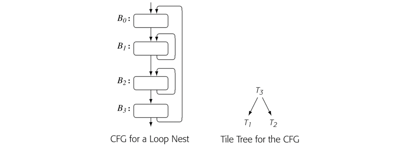
In this scheme, the allocator imposes a hierarchical model on the nodes of the CFG. In the model, a tile represents one or more CFG nodes and the flow between them. Tiles are chosen to encapsulate loops. In the CFG shown in the margin, tile $T_1$ consists of $\{B_1\}$. Tile $T_2$ consists of $\{B_2\}$. Tiles nest; thus, tile $T_3$ contains $\{B_0,T_1,T_2,B_3\}$. The tile tree in the margin captures this relationship; $T_1$ and $T_2$ are siblings, as well as direct descendants of $T_3$.

The hierarchical allocator performs control-flow analysis to discover loops and group blocks into tiles. To provide a concrete representation for the nesting among the tiles, it builds a tile tree in which subtiles are children of the tile that contains them.

Next, the hierarchical allocator performs a bottom-up walk over the tile tree. At each tile, $T_i$, it builds an interference graph for the tile, performs coalescing, attempts to color the graph, and inserts spill code as needed. When it finishes with ${\gamma }_i$, the allocator constructs a summary tile to represent ${\gamma }_i$ during the allocation of ${\gamma }_i$'s parent. The summary tile takes on the LiveIn and LiveOut properties of the region that it represents, as well as the aggregate details of allocation in the region--the number of allocated registers and any PR preferences.

Once all the tiles have been individually colored, the allocator makes a top-down pass over the tile tree to perform assignment--that is, to map the allocation onto PRs. This pass follows the basic form of the global allocator, but it pays particular attention to values that are live across a tile boundary.

The bottom-up allocation pass discovers LRs one tile at a time. This process splits values that are live across tile boundaries; the allocator introduces copy operations for those splits. The split points isolate spill decisions inside a tile from register pressure outside a tile, which tends to drive spills to the boundaries of high-pressure tiles.

Of course, the allocator could run a postal- location coalescing pass over the allocated code.

Cross-tile connections between live ranges become copy operations. The allocator uses a preferencing mechanism similar to biased coloring to remove these copies where practical (see Section 13.5.1). The same mechanism lets the allocator model requirements for a specific PR.

Experiments suggest that the hierarchical allocator, with its shorter live ranges, produced slightly better allocations than a straightforward implementation of the global coloring allocator. Those same measurements showed that the allocator itself used more compile time than did the baseline global coloring allocator. The extra overhead of repeated allocation steps appears to overcome the asymptotic advantage of building smaller graphs.

13.6 Summary and Perspective

Because register allocation is an important part of a modern compiler, it has received much attention in the literature. Strong techniques exist for both local and global allocation. Because many of the underlying problems are NP-hard, the solutions tend to be sensitive to small decisions, such as how ties between identically ranked choices are broken.

Progress in register allocation has come from the use of paradigms that provide intellectual leverage on the problem. Thus, graph-coloring allocators have been popular, not because register allocation is identical to graph coloring, but rather because coloring captures some of the critical aspects of the global allocation problem. In fact, many of the improvements to coloring allocators have come from attacking the points where the coloring paradigm does not accurately reflect the underlying problem, such as better cost models and improved methods for live-range splitting. In effect, these improvements have made the paradigm more closely fit the real problem.

Chapter Notes

Register allocation dates to the earliest compilers. Backus reports that Best invented the algorithm from Section 13.3 in the mid-1950s for the original Fortran compiler [27, 28]. Best's algorithm has been rediscovered and reused in many contexts [39, 127, 191, 254]. It best-known incarnation is as Belady's offline page-replacement algorithm, Min[39]. Horwitz [208] and Kennedy [225] both describe the complications created by clean and dirty values. Liberatore et al. suggest spilling clean values before dirty values as a compromise [254].

The connection between graph coloring and storage-allocation problems was suggested by Lavrov [250] in 1961; the Alpha project used coloring to pack data into memory [151, 152]. Schwartz describes early algorithms by Ershov and by Cocke [320] that focus on using fewer colors and ignore spilling. The first complete graph-coloring allocator was built by Chaitin et al. for IBM's PL8 compiler [80, 81, 82].

The global allocator in Section 13.4 follows Chaitin's plan with Briggs' modifications [57, 58, 62]. It uses Chaitin's definition of interference and the algorithms for building the interference graph, for coalescing, and for handling spills. Briggs added an SSA-based algorithm for live range construction, an improved coloring heuristic, and several schemes for live-range splitting [57].

The treatment of register classes derives from Smith, Ramsey, and Holloway [331]. Chaitin, Nickerson, and Briggs all discuss achieving some of the same goals by adding edges to the interference graph to model specific assignment constraints [60, 82, 284].

The notion of coloring disjoint subgraphs independently follows from Smith, Ramsey, and Holloway. Earlier, Gupta, Soffa, and Steele suggested partitioning the graph into independent graphs using clique separators [184] and Harvey proposed splitting it between general purpose and floating-point registers [111].

Many improvements to the basic Chaitin-Briggs scheme have appeared in the literature and in practice. These include stronger coalescing methods [168, 289], better methods for spilling [40, 41], register scavenging [193], rematerialization of simple values [61], and live-range splitting [107, 116,244]. Register promotion has been proposed as a preallocation transformation that rewrites the code to increase the set of values that can be kept in a register [73, 77, 258, 261, 315]. DasGupta proposed a precise incremental update for coalescing and spilling, as well as a faster but somewhat lossy update [124]. Harvey looked at coloring spill locations to reduce spill memory requirements [193].

The SSA-based allocators developed from the independent work of several authors [64, 186, 292]. Both Hack and Bouchez built on the original observation with in-depth treatments [53, 185]. Linear scan allocation was proposed by Poletto and Sarkar [296]. The hierarchical coloring scheme is due to Koblenz and Callahan [75, 106].